The Flare Star GJ 3685A

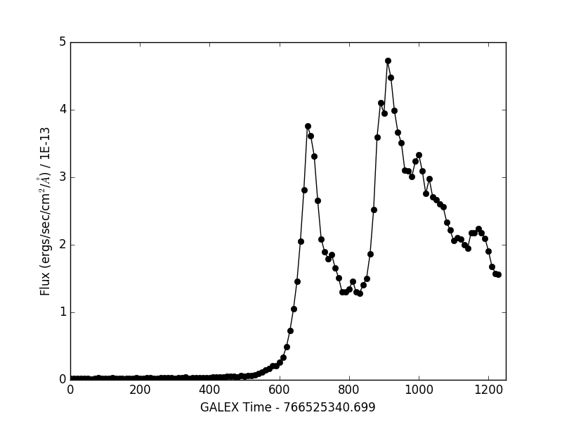
GJ 3685A is a flare star that underwent a double-flaring event while GALEX was observing. In this short exercise, we will create a plot of this event using gAperture. Below is the python script you will make.

import gPhoton

def main():
    gPhoton.gAperture(band='NUV', skypos=[176.91975, 0.25561], stepsz=10.,
	          csvfile='gj_3685a_lc.csv', radius=0.012,
                  annulus=[0.013,0.016],
	          trange=[766525335.,766526573.])

if __name__ == '__main__':
    main()

In our call to gAperture, we specify we would like to make a lightcurve using the NUV data via the "band" parameter. The coordinate of the center of our aperture is given in the "skypos" parameter. The "stepsz" parameter is used to make a lightcurve with 10-second sampling. The output file made by gAperture we will written to a file called "gj_3685a_lc.csv".

Our photometric aperture will be 0.012 degrees (43.2 arcsec), while our annulus for background subtraction will have inner and outer radii of 0.013 and 0.016 degrees (46.8 and 57.6 arcsec). Important Note #1: gAperture uses degrees for the photometric aperture and background annuli. The time range to extract data should start at GALEX timestamp 766525335. and end at GALEX timestamp 766526573. Important Note #2: gPhoton uses GALEX timestamps when specifying time ranges. A GALEX timestamp "t_GALEX" = t_UNIX - 315964800. A UNIX timestamp t_UNIX = the number of elapsed seconds since January 1, 1970. You do not need to specify a time range when you run gAperture, but in our example, we know when the flare occurs, so we focus only on that time range. If no trange is specified, gAperture will use all available data.

If you were to create the above python script in a file called "myscript.py" and then executed it from the Unix command line as "python myscript.py", you will create a comma-separated text table called "gj_3685a_lc.csv". You could then read this text table in using your favorite method, and if you were to plot the column "t_mean" (mean time per bin) on the x-axis and "counts" (photon events per bin) on the y-axis, you will see a figure similar to the one below showcasing the double flare event. You could also plot, for example, "flux_bgsub" (calibrated intensity per bin) on the y-axis, which would show the background-subtracted flux.