


 Follow Us
gPhoton Gotchas: Things To Be Aware Of When Analyzing Your Results
Back To gPhoton HomepageFUV Absolute Flux Discrepancies For CAI Data
When comparing fluxes from gPhoton against those available in the mission-produced MCAT, we have found a discrepancy for sources observed in CAI mode. The exact source is yet to be determined, but the largest effect (10-15%) seems to be limited to FUV data from the first three legs of the dither pattern. There is also a 2% bimodality across all legs. We will be adding a flag in a future build to indicate if the data you are looking at comes from a CAI observation.
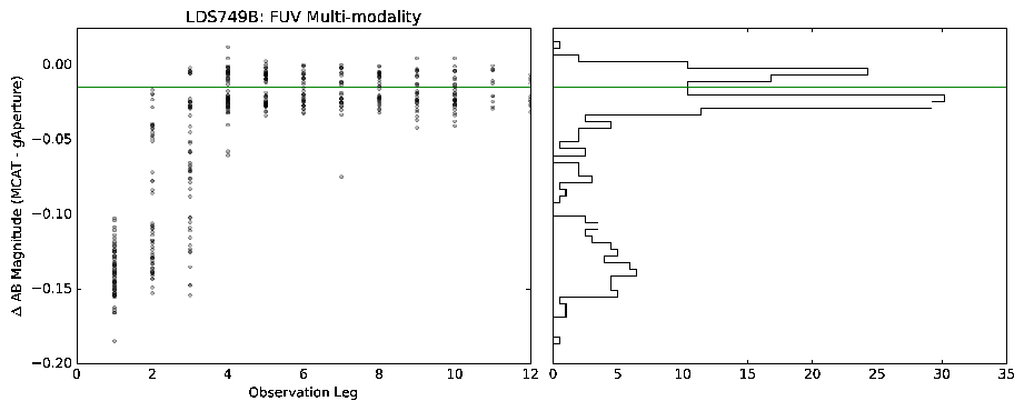 Plot of MCAT mag. - gPhoton mag. for the white dwarf calibrator LDS749B. The largest discrepancies occur in the first three legs of the dither pattern.
Dips Caused By Hotspot Masks
If your source passes over a masked hotspot, it can sometimes manifest in a way that looks like a very short duration transiting object. We have added a check to the software that will flag any bins that include data near a known hotspot. If you mask any bins with FLAG != 0, this will avoid many hotspot problems, but users should be cautions when analyzing any flux decreases to verify there are no unmasked hotspots. Recommended checks include creating gPhoton image sequences to look for hotspots visually, or to create plots of the raw photon event detector positions using the returned structure from gAperture (though note the latter requires you to run gAperture as an imported module).
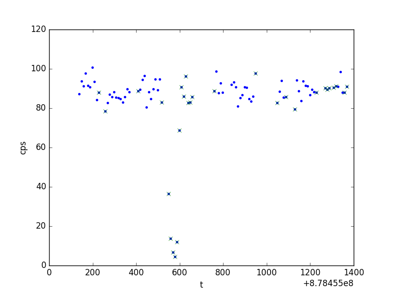 Light curve of LDS749B in NUV from gPhoton. The dip near t=600 looks like a transiting planet signal, but is actually caused by the source passing through a hotspot. Points marked with an 'x' are flagged by gPhoton to include this warning.
Correlated Flux Variations
Users should always check for correlations with other parameters when flux variability is seen. While this is one of gPhoton's main strengths, there are several other sources of variability that are non-astrophysical. If you see single-bin flux decreases, always check that the bin's effective exposure time is not significantly lower than other bins. Sometimes flux variability is strongly correlated with detector position, especially if the target moves over a large range during the dithers.
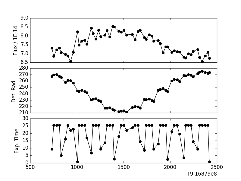 Example of correlated flux variation. In this case, the intra-visit flux variation is clearly related to the detector source position (middle panel), and is almost certainly non-astrophysical. Also notice there are some bins with low effective exposure time, often the first and/or last bins in a given dither position, so be sure to check the deffective exposure times for any bins where you see flux changes.
Flux Uncertainties
The light curve files produced by gAperture include an estimate of flux uncertainties, produced by adding the counting errors in the aperture and background annulus in quadrature, scaled to the area of the aperture. Any additional sources within the aperture or background annulus will produce poor uncertainty estimates. Users are encouraged to check for any additional sources within the apertures or background annulus by making deep coadd images. Future work will include better modeling of the imaging chain as a means to more accurately propagate uncertainties.
Effective Field-of-View / Detector Edge Effects
The GALEX detector edges tend to produce data of inconsistent or lower quality ("edge effects"). To minimize this, the tools restrict analyses to the inner 1.1 degrees of the 1.25 degree detector by default. If you find an inconsistency between the coverage reported by gPhoton and coverage reported elsewhere -- e.g. the MCAT -- then it may be due to this edge trimming. The effective detector size used by the gPhoton tools can be adjusted with the --detsize command line parameter, but analyze any resulting data with extra suspicion; assume that there are "unknown unknowns" contributing to the signal.
Similarly, data near the edge of the _virtual_ detector (as defined by --detsize in gPhoton) might cross over this boundary as the spacecraft moves during an observing sequence, and the flux may vary wildly as a result, so be aware that this could happen. A warning flag in cases like this will be added to gAperture soon.
Intra-Visit Variability Significance
The intra-visit level variability of GALEX has not been explored very much. We're still trying to understand the data at this level and, in particular, how to assess when observed variability is due to a real astrophysical phenomenon as opposed to instrument or calibration effects. We're working on a tool to "sanity check" data, but in the meantime we suggest the following strategies:
- Is the variation larger than 3 (or even 1) sigma, assuming Gaussian counting statistics? If not, it's highly suspect.
- Does the variation correlate in the time domain with effective exposure time (exptime), detector position (detx, dety, detrad), or response? If so, it is very likely a detector effect.
- Does the variation appear in light curves constructed with different choices of time bin size? If so, it is more likely to be real. We suggest starting with 30 second bins, and then trying 10 seconds or 60 seconds, although what constitutes a "good bin size" will depend on the brightness of your source.
Bins With Low Effective Exposure Time
Note that gAperture defines time bins as being regularly spaced (at the bin size) across all time, beginning at the arrival of the first valid data. For this reason, some bins (especially at the beginnings and ends of GALEX observations) might not be "full." This is handled by the exposure time correction, but results in lower counts, meaning higher error and a higher chance of extreme values. If you'd like to minimize this effect, use only bins where the effective exposure time (exptime) is >70% of the raw exposure time (t_end - t_start). Bins with effective exposure time < 50% are flagged, so as usual, users are encouraged to treat any bins with a non-zero flag with extra degrees of caution and analysis. If sufficient need is demonstrated, we may add options for different ways of defining bins (e.g. by maximizing coverage in each bin, or aiming for equal signal-to-noise in each bin).
Effective Exposure Time vs. Time Plots
The GALEX spacecraft was in Low Earth Orbit (LEO) and observed on the night side of each orbit (a so-called "eclipse"). Stray light or airglow from Earth's atmosphere was, and is, detectable within the data, and manifests as high global counts at the beginning and end of each eclipse, parabolic in shape. Because gPhoton estimates the detector deadtime correction based upon global count rates, this effect can sometimes also be seen when plotting the effective exposure time as a function of time (except inverted, because higher global counts result in more dead time and therefore less effective exposure), so be aware of this when making plots of effective exposure time for each bin.
Course Sun Pointing Event
In NUV data taken after the Course Sun Point (CSP) event, a small fraction of all events are mis-located along the detector y-direction. For brighter sources, this can manifest as the appearance of a "ghost" image that moves from observation to observation as a function of the spacecraft roll angle. They will often appear as sources that "move around" a target in animated images created by gPhoton. "New" sources that appear only in data collected after May 2010 should be viewed with extreme skepticism. Find more information here: http://www.galex.caltech.edu/wiki/Public:Documentation/Chapter_8
Back To Top
|
|
|