11.2.1 Ripple Correction

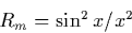
A distinctive feature of echelle gratings is the variation in sensitivity as a function of wavelength within a spectral order, commonly known as the blaze function. The adjustment applied to eliminate this characteristic is referred to as a ripple correction. The use of the term ``ripple'' becomes apparent when the net fluxes in successive orders are plotted as a function of wavelength. A series of scalloped or ripple patterns appear which must be corrected for prior to the application of the absolute calibration.

The ripple correction and all associated equations are defined in Cassatella (1996, 1997a, 1997b). The basic form of the ripple correction as a function of order number and wavelength is:

$$R_{m} = \sin^{2}x / x^{2}$$

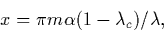
where x is expressed as:

$$x = \pi m \alpha (1 - \lambda_{c}) / \lambda,$$

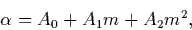
the $\alpha$ parameter is given as a function of order number:

$$\alpha = A_{0} + A_{1}m + A_{2}m^{2},$$

and the central wavelength corresponding to the peak of the blaze is:

$$\lambda_{c} = W_{0} / m + W_{1} T + W_{2} D + W_{3}.$$

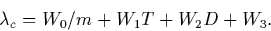
Note that unlike the SWP camera, the LWP and LWR ripple corrections do not exhibit a dependence of central wavelength on THDA; instead the observed central wavelengths vary linearly with time. In addition, the LWR $\alpha$ parameter evinces a bimodal behavior which has been fit with two separate functions (i.e., a linear and a quadratic polynomial). Here, m is order number, $\lambda$ is wavelength in Ångstroms, T is the THDA, and D is the observation date in decimal years. The ripple correction is applied to the net flux prior to the application of the heliocentric velocity correction to the wavelengths. The various ripple coefficients used in the above equations are given in Table 11.10 for each camera.

 

 

Coefficients LWP LWR SWP

$$m \geq 101$$ m < 101

A₀ 0.406835 3.757863 1.360633 0.926208

A₁ 0.01077191 -0.0640201 -4.252626e-3 0.0007890132

A₂ -5.945406e-5 3.5664390e-4 0.0 0.0

W₀ 230868.177 230538.518 137508.316

W₁ 0.0 0.0 0.0321729

W₂ -0.0263910 -0.0425003 0.0

W₃ 56.433405 90.768579 2.111841