7.10.3 Some Practical Considerations

  In most circumstances, a good range for i is from -5 to +5. Sometimes when a weak order is being extracted near a much stronger one, it is a good idea to adjust i to be a bit less expansive in the direction of the strong order, just in case the compensation is not perfect. It is usually true that an enlargement of the range in i to something greater than ± 5 does not buy enough gain in net signal-to-noise ratio to justify the risk of some extra residual cross talk from the adjacent orders.

From the standpoint of obtaining fair weight factors when the various measurements of $I_{m,\lambda}$ are combined, it is not particularly important that the general numbers for r, S_m-1, S_m, or S_m-1 are particularly accurate. However, for the analysis of absorption line optical depths, a correct value of r is critical. Sometimes, determining r is very difficult if there are no saturated lines in the vicinity. Most of the scattered light comes from the echelle grating. Thus, as one might expect, the levels of r are correlated with the brightness of the order that is being extracted. One way to check that an estimate of r is correct is to see if a vertical slice through an order, after r is subtracted, has a shape that agrees with [b(i) + b(i-10) + b(i+10)], as shown by the heavy line in the foreground of Fig. 12 (this assumes that the derivation of b is correct and universal thoroughout the format).

On some rare occasions, spectral lines appear to be somewhat slanted in the direction: ``\''. This behavior is probably a result of the astigmatism not being perfectly vertical. However, this effect does not appear all of the time, for reasons that are not clear. In extraction, one must be alert for this effect and stagger the sampling in a horizontal direction to obtain the best wavelength resolution.

When combining extractions from groups with different instrument pointing offsets (for a given echelle setting), it is again important to utilize the principle of keeping track of estimated errors and using them to determine relative weights for intensities, as discussed at the end of §7.10.2. Because of the pointing offsets, the spectral ranges will differ somewhat. It is a good idea to avoid sudden discontinuities that inevitably arise across the boundary of where one of the images stops on top of the coverage of another (because of the usual unavoidable systematic errors). One way to do this is to let the extraction of each image terminate gently by artificially multiplying the errors in short intervals near the ends by 1/H, where H is a Hanning window function.

 

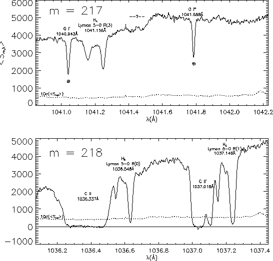
Figure 13: Extractions of two orders near the middle of Fig. 11. Associated with every value of $\langle S_{m,\lambda}\rangle$ plotted by the main curve, there is a computed error $\sigma ( \langle S_{m,\lambda}\rangle )$, as given by Eq. 14. The dotted line at the bottom of each panel represents the amplitude of 10 times this error. This noise level is relatively constant over all wavelengths because exposures with different pointing offsets are combined here. The noise level prediction line for a single stack of exposures, such as that shown in Fig. 11, would show increased levels over regions covering the holes in the photocathode sensitivity and upticks at the positions of the two bad columns.