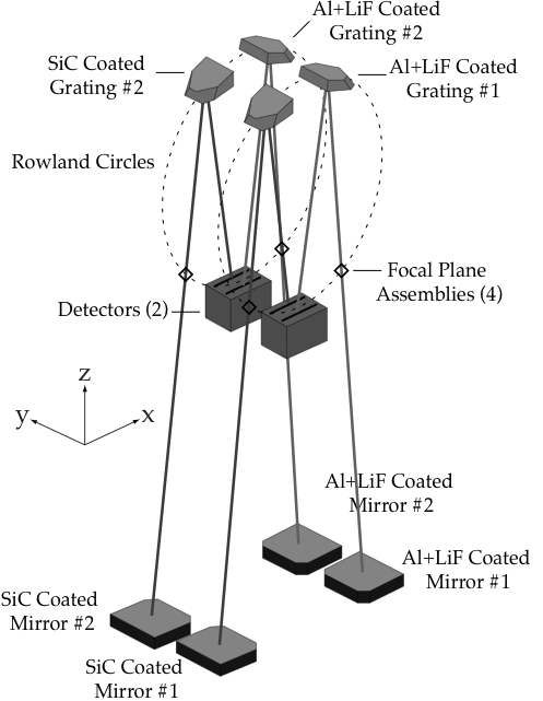
Optical layout of the FUSE instrument showing the 4-channel design.
|
|
To understand FUSE data, the "Intermediate" and "Advanced" users need to acquire some familiarity with the instrument and data acquisition. Thus, this section gives a brief description of these subjects. More details are given in Moos et al. (2000), Sahnow et al. (2000), and in the Instrument Handbook (2009).
The FUSE instrument (Figure 2.1) was a Rowland circle design consisting of four separate optical paths, or channels. A channel consists of a telescope mirror, a Focal Plane Assembly (FPA, which contains the spectrograph apertures), a diffraction grating, and a portion of a detector. The channels must be co-aligned to optimally observe a single target across the full FUSE bandpass. At the focal plane of the telescope, ∼90% of the light in the point spread function (PSF) lies within a circle of diameter 1.5″.
Two of the four channels used mirrors and gratings coated with SiC (to
maximize sensitivity for
![]() λ
λ
![]() 1000 Å,
and the other two
were coated with aluminum and LiF (to maximize sensitivity for
1000 Å,
and the other two
were coated with aluminum and LiF (to maximize sensitivity for
![]() 1000 Å,
). The four channels comprise two nearly identical
"sides" of the instrument, where a side consists of one LiF and one
SiC channel, each producing a spectrum which falls onto a single detector.
Each channel has a bandpass of about 200 Å. Thus, at least two channels
are required to cover the
∼290 Å wavelength range of the instrument.
1000 Å,
). The four channels comprise two nearly identical
"sides" of the instrument, where a side consists of one LiF and one
SiC channel, each producing a spectrum which falls onto a single detector.
Each channel has a bandpass of about 200 Å. Thus, at least two channels
are required to cover the
∼290 Å wavelength range of the instrument.
Figure 2.1 also shows the orientation of the instrument prime coordinate system (X,Y, Z). The two LiF channels are on the +X side of the instrument, which is always kept in the shade (i.e., the −X side was always facing toward the sun). This orientation minimizes the amount of sunlight that can make its way down the baffles surrounding the LiF channels. Minimizing stray light in the LiF channels was crucial to the operation of the Fine Error Sensor (FES) guidance camera, which operated at visible wavelengths (see Chapter 5). The orientation of the satellite was biased by several degrees in roll around the Z axis in order to keep the radiator of the operational FES in the shade.
Each telescope focused on an FPA that served as the entrance aperture for its spectrograph. An FPA was a flat mirror mounted on a two-axis adjustable stage which contained three apertures. The apertures were not shuttered, so whatever light fell on them was dispersed by the gratings and focused onto the detectors.
The orientation of the three apertures is depicted in Fig. 2.2, and their properties are summarized in Table 2.1. The HIRS aperture ensured maximum spectral resolution, minimum sky background and sometimes allowed for spatial discrimination for extended objects or crowded stellar fields. However, it blocked part of the point spread function, and small, thermally induced mirror motions often led to the loss of all light from one or more channels during an observation. The MDRS aperture, with stable mirror alignment, provided maximum throughput and a spectral resolution comparable to the HIRS aperture for a point source with only slightly more airglow contamination than HIRS. However, it too, was susceptible to thermal drifts of the separate channels. The LWRS aperture was the least sensitive to alignment issues, but it allowed the largest sky background contamination. Although image motion could degrade the resolution of LWRS spectra, this was largely corrected by the pipeline processing for TTAG data. The LWRS aperture was also used to observe faint extended objects, producing a filled-aperture resolution of ∼100 km s -1. LWRS was the default aperture throughout most of the mission because of the thermal image motions that occurred on orbit.
In addition, a target could also be placed outside the apertures at the reference point (RFPT), which did not transmit light. When a target was placed at the RFPT, the three apertures sampled the background sky nearby.
Each FPA could be moved independently in two directions. Motion tangential to the Rowland circle, which is roughly in the dispersion direction, and perpendicular to the apertures. These motions allowed co-alignment of the channels and permitted focal plane splits (FP splits, see Chapter 7) for high signal-to-noise ratio observations of bright targets. Motion in Z enabled focusing of the apertures with respect to the mirrors, spectrograph grating, and detector.
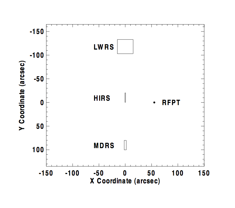 |
| Aperture | Name | Dimensions | Number(an)+ | Comments | X Position | Y Position |
|---|---|---|---|---|---|---|
| Medium resolution | MDRS | 4.0 × 20″ | 2 | - | 0.00″ | +90.18″ |
| High resolution | HIRS | 1.21 × 20″ | 3 | - | 0.00″ | 10.27″ |
| Low resolution | LWRS | 30 × 30″ | 4 | Nominal Aper. | 0.00″ | -118.07″ |
| Reference Point | RFPT | - | 4 | - | 55.18″ | 0.00″ |
| + Aperture naming convention. an =1 corresponded to the PINHOLE aperture which was never used. | ||||||
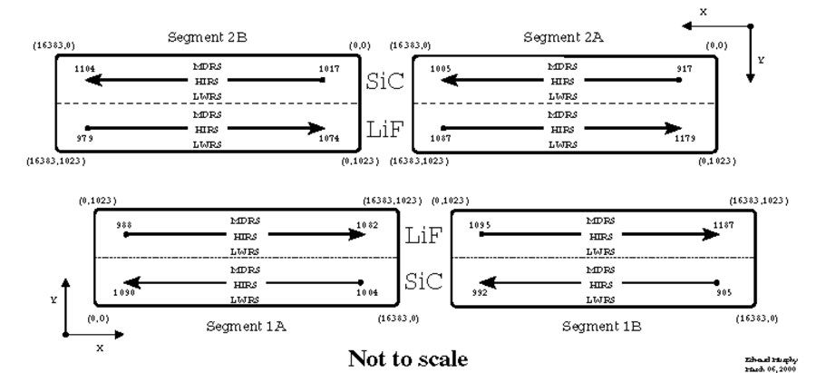
FUSE spectra covered
905![]() &lambda
&lambda![]() 1187Å. The spectra
from each of its four channels were imaged onto two microchannel plate
detectors. Each detector had one SiC and one LiF spectrum imaged onto it,
thereby covering the entire wavelength range. The two channels imaged on
each detector were offset perpendicular to the dispersion direction to
prevent them from overlapping. The dispersion direction of the SiC and LiF
spectra were in the opposite sense (see Figure 2.3). Each
detector consisted of two functionally and physically independent segments
(A and B)
separated by a small gap. To ensure that the same wavelength region did
not fall into the gap on both detectors, the detectors were offset slightly
with respect to each other in the dispersion direction.
Table 2.2 lists the wavelength
coverage for each of the eight detector segment and channel combinations.
Nearly the entire wavelength range was covered by more than one channel,
and the important 1015-1075 Å range was covered by all four, providing
the highest effective area and the greatest redundancy.
1187Å. The spectra
from each of its four channels were imaged onto two microchannel plate
detectors. Each detector had one SiC and one LiF spectrum imaged onto it,
thereby covering the entire wavelength range. The two channels imaged on
each detector were offset perpendicular to the dispersion direction to
prevent them from overlapping. The dispersion direction of the SiC and LiF
spectra were in the opposite sense (see Figure 2.3). Each
detector consisted of two functionally and physically independent segments
(A and B)
separated by a small gap. To ensure that the same wavelength region did
not fall into the gap on both detectors, the detectors were offset slightly
with respect to each other in the dispersion direction.
Table 2.2 lists the wavelength
coverage for each of the eight detector segment and channel combinations.
Nearly the entire wavelength range was covered by more than one channel,
and the important 1015-1075 Å range was covered by all four, providing
the highest effective area and the greatest redundancy.
 |
The SiC channels had an average dispersive plate scale of 1.03 Å/mm while the LiF channels had a scale of 1.12 Å/mm (Moos et al. (2000)). Coupled with the detector pixel size, this resulted in a scale of ∼6.7 mÅ/pixel in the LiF channel and ∼6.2 mÅ/pixel in the SiC channel (in the X or dispersion direction).
The optical design of the FUSE spectrographs introduced astigmatism. The astigmatic height of FUSE spectra perpendicular to the dispersion was significant; the dispersed image of a point source had a vertical extent of 200 - 900 μm, or 14 - 63″, on the detector. An extended source filling the large aperture was as large as 1200 μm, or 100 ″ This vertical astigmatic height was a function of both wavelength and detector segment. This meant that the spatial imaging capability of FUSE was extremely limited. For the spectral region near the minimum astigmatic heights in each spectrum, there was marginal spatial information ( >10″ ) , but to recover this requires careful, non-standard processing. The minimum astigmatic points were near 1030 Å on the LiF channels and near 920 Å on the SiC channels.
Moreover, spectral features showed considerable curvature perpendicular to the dispersion, especially near the ends of the detectors where the astigmatism was greatest. This astigmatism is corrected for in the data prior to collapsing it into a 1-D spectrum (see Chapter 7 and the Instrument Handbook (2009) for details).
| Channel | Segment A | Segment B |
|---|---|---|
| SiC 1 | 1003.7 - 1090.9 | 905.0 - 992.7 |
| LiF 1 | 987.1 - 1082.3 | 1094.0 - 1187.7 |
| SiC 2 | 916.6 - 1005.5 | 1016.4 - 1103.8 |
| LiF 2 | 1086.7 - 1181.9 | 979.2 - 1075.0 |
| a Note the redundancy especially in the 1015-1075 Å range. | ||
The FUSE instrument included two photon-counting microchannel plate (MCP) detectors with delay line anodes. Each detector, which was a single optomechanical unit, consisted of two functionally independent segments. Each segment could be separately controlled since it had its own high voltage control, anode, and digitizing electronics. The two segments in a detector were separated by a several millimeter gap, which was not sensitive to photons. In order to ensure that the same wavelength interval did not fall into the gap on both detectors, the two detectors were offset by several degrees with respect to each other along the Rowland circle. The two detectors were designed to be identical, although variations in MCP properties and electronics adjustment led to a number of minor differences between them.
Each segment included a stack of three MCPs with its own double delay line anode. A photon incident on the front surface of one of the MCPs resulted in a ∼107 electrons at the bottom of the stack. This charge cloud was collected by the anode and event locations were determined by measuring the time propagation along the delay line in the spectral dispersion direction and by charge division in cross dispersion. The measured positions were then digitized into 16,384 × 1024 pixels. Thus the FUSE "pixels" were not physical objects, but rather the digitization of analog measurements.
On all segments, the X (dispersion dimension) pixel size was ∼6 μm. However, the Y (orthogonal to the dispersion) pixel size was different for the different detector segments in the raw data (in the calibrated data, all segments were adjusted to a common Y scale). For segments 1A and 1B, the Y pixel size was ∼10 μm, and it was somewhat larger for segments 2A and 2B. However, the detector resolution (i.e., the ability of the electronics to locate an event) was ∼ 20 × 80 μm. Hence, the detector resolution was oversampled by a factor of 4 or more.
The two units were designated Detector 1 and Detector 2, and the segments were labeled A and B. Thus, the four segments were denoted as 1A and 1B (on side 1 of the instrument), and 2A and 2B (on side 2) (see Fig. 2.3).
Because X and Y
coordinates were calculated from timing and voltage
measurements of the charge cloud, the detector coordinate system was subject
to distortions caused by temperature changes and
other effects. To track changes in this distortion as a function of time,
electronic "stim pulses" were injected
into the detector electronics at the beginning and end of each exposure.
The stim pulses appear near the upper
left and upper right corners of each detector segment, outside of the active
spectral region. The stim pulses were well placed for tracking changes in
the scale and offset of the
X (dispersion) coordinate, but they were not well enough
separated in
Y (spatial) to track scale changes along that axis. CalFUSE used
the stim positions to correct for thermal effects.
Detector Background: Microchannel plates possess an inherent background rate, which is due mainly to beta decay in the MCP glass. On orbit, cosmic rays added to this to give a total rate of ∼0.5 counts cm -2 sec-1. Since there was no shutter in the optical system, airglow emission, which constantly changed, also contributed to the overall background.
Stim Lamp: A stimulation, or "stim" lamp was located just below the internal spectrograph baffles on each side of the instrument, and about 1.25 m above each detector. These lamps were used in orbit as an aid in calibration.
Counters: Several types of event counters were calculated by the FUSE detectors in parallel with all observations. Two counters that are important for calibration purposes are the Fast Event Counter (FEC), which measures the count rate at the detector anode, and the Active Image Counter (AIC), which yields count rates at the back end of the detector electronics. These count rates were used by CalFUSE to monitor a variety of effects, to screen the data for various anomalies, and to determine dead time corrections.
More details about the detector subsystem and its performance can be found in the FUSE Instrument Handbook (2009) and the references provided therein.
The front surface of the two LiF FPAs had a reflective coating, and light not passing through the apertures was reflected into a CCD camera for each side. Images of the field of view (FOV) around the apertures were used for acquisition and guiding by a camera system called the Fine Error Sensor (FES). The FES cameras imaged a 19′ × 19′ field around (but not centered on) the apertures. Each FES imaged the FPA onto a quadrant of a 1024 × 1024 pixel CCD, which was masked to a 512 × 512 pixel image, with pixels of 24 × 24 μm and a plate scale of 2.55″ pixel-1 Only one of the two FESs was used at a time. The FWHM of the FES PSF was typically ∼5″. More details can be found in Chapter 5 and in the Instrument Handbook (2009).
The four-channel design of FUSE allowed for redundancy in spectral coverage and improved total instrument throughput. With multiple spectra overlapping different wavelength regions, the user can cross-check spectral measurements from the independent spectrographs and, in theory, improve the signal-to-noise of the data. This has to be done carefully, however, since the spectra have different resolutions, wavelength shifts, and small scale structure due to differing detectors and optical effects. While narrow apertures were available with FUSE, most observations used the large LWRS aperture, for which the spectrographs operated in a slitless mode. In this case, wavelength accuracy and resolution were dependent on how well the target was centered in the aperture and how stable the position was maintained during the observation. Because there were four channels, accurate target pointing had to be achieved in four apertures simultaneously for best results.
Due to several hardware problems in the instrument and spacecraft, target placement was not completely stable during most exposures. Movements of the target and spectra often induced errors in measured fluxes, absolute wavelengths, and resolution. Most of these effects were corrected by processing in the CalFUSE pipeline software especially for Time-Tag mode data (see below). Nonetheless, the user of FUSE data should be aware of these problems since the corrections are imperfect (see Chapter 7).
Thermal effects that occurred with the instrument included: mirror misalignment and motion, and motions of the spectrograph gratings. Gradual failure of the spacecraft gyroscopes and reaction wheels over the course of the mission degraded the pointing control at times. These problems are discussed in the next sections.
Coalignment of the FUSE channels was difficult to maintain because the telescope mirror benches were thermally coupled to the space environment external to the instrument. Thermal expansion and contraction of the baffles is suspected to have moved the optical bench on which the mirrors were mounted, causing a shift of the sky viewed by each aperture. If the thermal environment of a target was significantly different than the previous one, there could be a secular shift of the mirrors over several hours. On top of this, there would be smaller orbital variations as FUSE went in and out of sunlight. The shifts could be large enough to move the target out of the aperture for a channel, especially for HIRS and MDRS observations. The SiC mirrors showed larger shifts than the LiF ones since they were on the sunlit side of the instrument. The channel with the best alignment was always the LiF side used with the guiding FES. For that channel, any shift of the star field would automatically be detected and removed by the spacecraft attitude control system. Prior to 12 July 2005, LiF1 was the guiding channel, and consequently, the LiF1 spectra where well centered in the aperture, resulting in the best wavelength and photometric accuracies. After that, LiF2 was used for guiding (Table 2.3).
Several observing strategies were implemented to help maintain alignment. An empirical model was devised to predict the alignment based on target orientation with respect to the Sun and Earth and prior history of pointing. At the beginning of an observation, the mirrors or FPAs would be adjusted to a predicted setting. If the change in thermal environment was expected to be large, the instrument would be allowed to thermalize until the target was predicted to be within the LWRS aperture. Residual motions associated with the completion of the thermalization process are removed in the pipeline processing. Sky background observations (e.g., S405/S505 programs) were sometimes acquired during long thermalization periods.
Periodically, an alignment procedure would be run, which scanned the instrument across a star to locate the aperture edges (e.g., M112/M212 programs). After assessment on the ground, the mirrors would be adjusted into alignment. Finally, if the MDRS or HIRS apertures were being used, one or more target peakups would be scheduled even multiple times per orbit to recenter the FPAs before starting exposures. This was a time-consuming and operationally complex activity and was only performed when deemed necessary for the science program.
For TTAG observations, CalFUSE applied a model for expected mirror motions during an orbit and performed photon position corrections for the non-guiding channels for point sources. This model was developed empirically from on-orbit measurements of actual thermal misalignments. The FPA position reading at the beginning of an exposure was used to set the wavelength zero point for a channel. No corrections of fluxes were made for the target being outside the apertures. For HIST data, exposures were kept short enough to minimize any smearing due to thermal motions during a single exposure. Individual exposures could be aligned before co-adding to remove any detected offsets.
Besides movement of the telescope mirrors within the instrument, the spectrograph gratings also rotated slightly with changes in thermal environment. This caused the spectra to move on the detector. Since airglow emission lines shifted as well, an empirical model could be developed to predict the orbital motions and was used by CalFUSE to remove these shifts.
FUSE was built with six gyroscopes and four reaction wheels, and at the beginning of the mission, the Attitude Control System (ACS) could obtain subarcsec pointing stability during an exposure. Pointing errors were much smaller than all the apertures and were an insignificant contributor to wavelength offsets and spectral resolving power. Except for rare circumstances, such as loss of guide stars during an exposure, guidance stability was not an issue when a user worked with the science data.
As the mission progressed, ACS hardware components began to fail and maintaining stable pointing
at a target became more difficult. As with the telescope mirror motions, a target could wander
around inside the aperture during an exposure, degrading the spectral resolution and wavelength
accuracy, or leave the aperture entirely, sometimes to return later in the exposure. But unlike
the instrument motions, the location of the target can be estimated from the pointing information,
and the data corrected in ground processing. Since the correction is an estimate, though often an
accurate one, the user needs to be vigilant with FUSE spectra. Details about guiding are found in
the jitter file associated with each exposure (Section 5.2). Table 2.3 lists the dates
when significant changes were made to FUSE pointing control.
The Instrument Data System (IDS) was a computer processor that controlled the FUSE instrument. The IDS communicated with all instrument subsystems, and was responsible for controlling all instrument functions, including thermal control, actuators on the mirror assemblies and FPAs, and detector and Fine Error Sensor (FES) operations. It received data from the FUV detectors and FES, and packaged them for transmission to the onboard solid-state recorder. The IDS also collected the housekeeping telemetry (temperatures, voltages, etc.) from these subsystems, packaged them, and sent them to the recorder.
The IDS played a crucial role in the pointing performance of the instrument. After a slew, it processed the FES image of the new field and determined the pointing based on comparison with a star table uplinked from the ground for each observation. This measured pointing was sent to the spacecraft Attitude Control System (ACS) to update the current pointing and the spacecraft was slewed to the desired target position. Once the FES acquired guide stars, it began sending centroid information for the guide stars to the IDS. The IDS computed the measured pointing vector (quaternion) once every second and sent it to the ACS to maintain pointing stability. Guiding was terminated prior to each occultation of the target by the earth. As long as guide stars had been acquired prior to entry into the South Atlantic Anomaly (SAA), guiding often proceeded through the SAA period even though observations were halted.
Although the FUSE detectors were photon-counting devices, memory considerations resulted in the science data being saved in two different ways. For each incident photon the detector X (14 bits) and Y (10 bits) positions, along with the pulse height (5 bits). A 32 bit word containing this information, along with detector and segment bits and one bit marking it as a photon event, was then constructed. An Active Image Mask was then applied. (The purpose of the mask was to allow the exclusion of detector regions which had very high count rates, e.g. due to a hot spot or other effect, that might overwhelm the science data bus. During the mission, however, no data needed to be excluded on any segment using the Active Image Mask.) The IDS collected the photon data from the detector and then stored it in memory as a photon list for lower count rates (time-tag or TTAG mode), or created a two-dimensional histogram of the data for higher count rates (histogram or HIST mode). For more details on detector data processing and masks, see the FUSE Instrument Handbook (2009).
When using photon address or time-tag (TTAG) mode, the position of each photon coming from the detector, along with its pulse height, was saved in IDS memory. Time markers were inserted into this data stream at a regular rate (typically once per second) by the IDS. Later, when the *fraw.fit files (see Section 4.2.1.1) were created by OPUS, the time taken from the preceding time marker was assigned to each photon event, so that raw TTAG data files include a floating point time, X (0 - 16383), Y (0 - 1023), and pulse height (0 - 31) for each photon. The data files include photon events from all apertures, along with background detector regions. One aperture in each channel contained the spectrum of the target, while the others only contained spectra of the sky plus airglow and detector background. Occasionally, in crowded fields, stars nearby the target object could enter a non-prime aperture and thus be recorded.
Data obtained in TTAG for very bright targets could not be transferred
fast enough resulting in partial data loss. Consequently, when the UV flux of a
target was expected to produce count rates larger than 2500 cps from all
detector segments combined, the IDS was commanded to
store the data in spectral image, or histogram (HIST) mode.
In this case, the photons were binned in
X and Y and the
arrival times and pulse heights of the photons were lost. The size and
positions of these bins were determined by the Spectral Image Allocation
(SIA) table, which was uploaded to the IDS before each HIST observation.
The SIA table was a buffer made up of 512 rectangles. The size of each
rectangle was 2048 pixels in
X and 16 pixels in Y. Thus, the 512
elements of the SIA table constitute an
8 × 64 image which spans the
16384 × 1024
elements of the detectors. The SIA table specifies
which of these rectangles should be saved (mask bit set "on" i.e., if
the IDS received a photon event from the detector whose
(X,Y) coordinates
map to a location in an active rectangle, then that photon event is stored
by incrementing a counter in a histogram bin at the specified binning.
The default histogram binning size was
1 × 8 (X,Y) detector pixels.
The default SIA table
specified storage of a region around the aperture containing the target,
and required
∼20 MB of storage for an orbit's worth of exposures.
Note that in HIST mode, only data taken
through the science aperture were recorded. Because Doppler
compensation was not performed on-board, HIST exposures times were kept
short to avoid losing spectral resolution and minimize smearing from thermal motions.
Typical HIST exposure times were
∼400 s. More information can be obtained in the
Instrument Handbook (2009.
A series of events impaired optimal use of the FUSE spacecraft and impacted the data acquisition and processing during those times. A list of the most significant events affecting FUSE data quality is given in Table 2.3 where Column (1) lists the chronology of these events since the FUSE launch; Column (2) gives a brief description of the events that took place; and Column (3) points to Notes to the table. A complete listing of such events can be found in the Instrument Handbook (2009).
| Date | Event | Notes |
|---|---|---|
| 24 June 1999 | Launched | ... |
| 12 December 1999 | LiF1 Focus Finalized | (1); (3) |
| 16 March 2000 | LiF2, SiCl,2 Focus Finalized | (1); (3) |
| 25 November 2001 | Yaw RWA failed | (2) |
| 10 December 2001 | Pitch RWA failed | (2); Science operations suspended |
| February 2002 | Two-wheel mode begins | Observations resumed |
| 03 February 2003 | Segment 2A HV confined | (4) |
| 31 July 2003 | Yaw IRU-B failed | (2); Gyroless control mode used |
| 27 December 2004 | Roll RWA failed | (2); Science operations suspended |
| March 2005 | One-wheel mode begins | Observations resumed |
| 12 July 2005 | LiF2 made default guiding channel | (3) |
| 12 July 2007 | Skew RWA failed | End of FUSE pointed observations |
| 18 October 2007 | Decommissioning | End of FUSE mission |
NOTES to table: