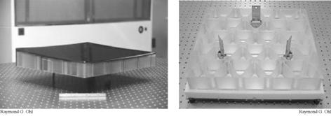
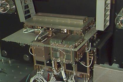
Figure 6‑1: Left: FUSE mirror resting face-up on flexures prior to integration into the mirror assembly. Right: Backside of the FUSE primary mirror illustrating the aggressive lightweighting of the Zerodur mirror substrate.
The primary mirror sections did not contain the vertex of the parent paraboloid. The vertex was about 34.5 μm from the edge of the mirror aperture in x (See Figure 6-32). The different grating incidence angles required to optimize the spectrograph channels for the two wavelength bands resulted in slightly different off-axis angles for the SiC and Al+LiF coated mirrors. The off-axis angles were defined by aperture stops placed over the surfaces of the mirrors. Otherwise, the mirrors are identical except for the coatings. The corners of each mirror were masked to match the grating apertures, whose outside corners were removed to satisfy space constraints of the ‘Med-Lite’ launch vehicle fairing. The resulting geometric area of each mirror was approximately 1330 cm2. These apertures were widely separated on the instrument optical bench, resulting in four parallel and separated optical axes. Selected mirror assembly specifications are listed in Table 6.1‑1. The point spread function (PSF) at the focal plane places ~90% of the light within a diameter of 1.5 arcsec.
| Mirror type | Off axis parabola |
| Substrate material | Zerodur |
| Size of clear aperture | 387′ 352 μm |
| Focal length | 2245 μm |
| Off axis angle (to optical center) | 5.3668° (SiC mirrors) 5.4678° (LiF mirrors) |
| Coatings | 2 mirrors with SiC 2 mirrors with Al+LiF |
Table 6.1‑1: FUSE Mirror Properties
The mirrors were fabricated from Zerodur, chosen for its low coefficient of thermal expansion (CTE). The blanks were aggressively weight-relieved: 70% of the substrate material was removed from each, leaving a triangular isogrid rib pattern with a 7.5mm-thick facesheet and a final mass of 7.7 kg (Figure 6‑1). This triangular rib structure provided a lightweight but very stiff substrate. SVG Tinsley Laboratories lightweighted the blanks and figured the mirrors into parabolas.
Figure 6‑1: Left: FUSE mirror resting face-up on flexures prior to integration into the mirror assembly. Right: Backside of the FUSE primary mirror illustrating the aggressive lightweighting of the Zerodur mirror substrate.
Each mirror is attached to the front of a honeycomb-sandwich intermediate plate by means of tangential-blade flexures, which minimize mounting-induced stresses and distortions and isolates the mirror from stress induced by adjustments of the actuators (Nikulla, 1997). The flexures are oriented with soft axes radial to the center of the mirror (Figure 6‑1 Right), and consist of titanium alloy blades attached to low-CTE Invar fittings. Each Invar fitting is bonded to a mirror rib. Three stepper-motor actuators are attached to the rear of the intermediate plate. This permitted independent tip, tilt, and focus control for on-orbit adjustment of each mirror (Figure 6‑2). The tip-tilt mechanism is used to provide rough alignment of the mirrors to the FPA entrance apertures.
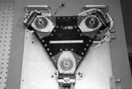
Figure 6‑2: Face-on view of mirror actuator assembly showing the three actuators and composite structure.
The instrument optical bench was constructed of hollow rectangular tubes and sheets composed of a graphite/cyanate ester composite material, designed to have a high strength-to-weight ratio, low CTE, and to insure dimensional stability over long integrations (200 kilo-second).
Individual pieces of the optical bench structure were bonded to form subassemblies that were joined by titanium fittings. Optical components were mounted to inserts built into the structure. Other components, such as the mounting plates for the electronics boxes, the baffles, contamination cover, etc., were mounted to the structure by flexures to avoid introducing any loads that might deform the structure and disturb the alignment of the optics. Exceptions to this practice, such as the lower baffle extensions, involved flexible materials that were not expected to apply significant loads. During thermal vacuum testing it was realized that mounting the contamination covers to the spectrographs resulted in undesirable motions of the grating bench. That mounting was modified and the new mounting validated in a second thermal vacuum test prior to launch. The decoupling of secondary hardware from the optical bench was not entirely satisfactory, however. The primary mirrors and gratings were found to move on orbital timescales once on-orbit. These motions, described in Section 5.2, were a significant complication to on-orbit operations.
Mechanical G-release, thermal expansion, and moisture desorption were expected to change the structure's dimensions significantly upon orbital insertion and slowly over the life of the satellite. Any errors in the placement of the mirror assemblies on the instrument optical bench would further misalign the mirrors with respect to the spectrograph (Conard et. al, 1999). Therefore to maintain alignment post-launch and throughout the mission, each mirror was equipped with precision actuators that permitted on-orbit mirror alignment.
Thermal control is maintained by heaters attached to the intermediate plates, which radiatively couple to the rear of the mirror substrates.
The temperatures of the optical elements were regulated by heaters mounted on their enclosures (“pie pans”), and on the intermediate plate in the case of the mirrors. The instrument thermal control system was always configured to maintain the temperatures of the optics at least two degrees C warmer than their surroundings to minimize the likelihood of contamination.
Optical testing and modeling of the FUSE primary mirrors were conducted toward a prediction of the on-orbit mirror point spread function (PSF) and its impact on spectrograph slit transmission. The image test was not meant to fully characterize the performance of the telescope mirrors in the FUSE bandpass. Rather, it was designed to insure that there were no severe problems with the flight mirrors and the implications of surface metrology data were understood. The test produced a data set which we used to validate our modeling and extrapolate a prediction into the FUSE bandpass with confidence.
Pre-launch measurements verified that the reflectivities of the optics exceeded their requirements of 32% for the SiC optics and 60% (λ > 1050Å) for the Al/LiF optics. Degradation of total system throughput of up to 20% per year was anticipated, but on-orbit performance was much better. The effective area of FUSE as a function of wavelength and time is presented in Figure 4‑2. Total throughput for the Al/LiF channels declined by less than 15% in the mid-wavelength band, and by ~25-30% in the long-wavelength band over the first three years, and was roughly stable thereafter. Performance degradation of the SiC optics differed: throughput declined at a roughly constant rate, falling by ~50% over 8 years. It is not possible to separate degradation of the primary mirrors from that of the gratings.
In addition to meeting reflectivity specifications (Oliveira et al. 1999), the fully assembled primary mirrors had an imaging requirement to contain 90% encircled energy (EE) at 100.0 nm in a diameter of 1.5 arcsec. This corresponded to a 16 micron diameter at the focal plane. To meet this requirement, FUSE established fabrication tolerances based on SOHO SUMER mirror heritage (Saha et al. 1996) and a modulation transfer function (MTF) analysis carried out at The Johns Hopkins University (JHU). The surface fabrication specifications were: figure error better than λ/40 RMS and λ /10peak-to-valley (P-V) at λ = 632.8 nm; midfrequency error less than 20 Å RMS over 10.0-0.1 mm spatial scales; and microroughness less than 10 Å RMS over 100-1 microns. These performance specifications were to ensure adequate transmission through the 1.25 × 20 arcsec, high-resolution spectrograph slit and instrument spectral resolution when using wider slits.
The in-flight mirror PSF performance was consistent with pre-flight measurements and model predictions (Ohl et al. 2000a, Ohl et al. 2000b). The mirror assemblies met the encircled energy requirement of 95% transmission through the 4 arcsecond MDRS aperture, and provided 90% transmission through the 1.25 arcsecond HIRS aperture, far-exceeding the 50% requirement.
In summary, the primary mirror assemblies were lightweight and adjustable in three degrees of freedom, maximized instrument reflective area in the bandpass, and met a stringent imaging requirement.
The position of each telescope mirror was adjustable through a Mirror Positioning Assembly (MPA). Each MPA (Figure 6‑3) consisted of three actuators controlled by one of two Mirror Assembly Electronics (MAE) packages, two thermistors, and one strip heater, with redundant heater elements on the side of the intermediate plate closest to the mirror. The heaters held the assembly to 22 degrees +/- 0.5 degrees C. Each MAE controlled a pair of mirror assemblies with one LiF coated mirror and one SiC coated mirror.
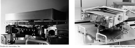
Figure 6‑3
Left: Dummy aluminum mirror with actuator assembly (ref Ohl).
Right: Full
flight mirror assembly, including pie-pan thermal enclosure and aperture stop.
Three actuators provided focusing and optical alignment for each of the four mirrors ( Figure 6‑4), enabling a focus resolution of 0.310 microns over a +/- 2.1 mm range and a tip/tilt resolution of 0.160 arcsec over a +/- 32.34 arcmin range. The “A” actuator controlled the rotation of the telescope mirror about the IPCS y-axis and consequently moved the target in the X-direction on the FPA (and the dispersion direction on the detector). The “B” and “C” actuators controlled the rotation of the telescope mirror about the IPCS X-axis. The combined motion of the “B” and “C” actuators adjusted the position of the target in the y-direction on the FPA. Equal motion of all three actuators moved the mirrors in the z-direction, or focus. Every movement of each actuator had to be tracked on the ground during the mission. Their range of motion is discussed in Section 6.7.5.1.
12.0pt'>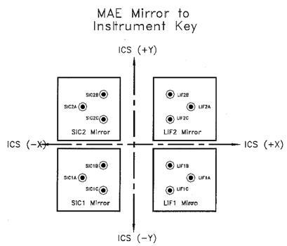
Figure 6‑4: The actuator locations relative to the mirrors and the IPCS coordinate frame.
The mirror assembly positioning actuators, each contained a stepper motor and an optical “soft stop” sensor that electrically interfaced with the appropriate MAE. The mirrors were positioned by an open-loop system. The initial on-orbit focus and alignment was determined from ground test. The MAEs had no memory, nor decision-making capability, nor were the absolute positions of the actuators telemetered. The specified stepper motor was commanded to move a certain number of steps in a specified direction, and the MAE attempts to comply with the command. Neither the MAE or the IDS was informed if a hard stop was encountered. The hard stop was also not telemetered. To facilitate alignment in the event knowledge of the mirror position was corrupted, each mechanism had a "reference position". This reference was a known position and, similar to the soft stops, was sensed using an optical disk encoder and therefore independent of commanding a known number of steps enabled.
In general, except for the "soft stop" function, the MAE did not know the current mechanism position. As a consequence, the ground software needed to maintain a record of the current expected actuator position and drive state of each of the twelve mechanisms. This record was updated each time one of the mechanisms was commanded.
To achieve initial alignment and focus, heavy usage of the MPAs was expected at the beginning of the mission, with only minor mirror adjustments expected later to compensate for structural changes from outgassing. Given this expectation for infrequent adjustments of the mirror positions, no position encoders were placed on the actuators and an on-board mirror motion manager, which could track mirror position through motion commands, was not developed. Post-launch, the four mirror channels (SiC1, SiC2, LiF1, and LiF2) were found to wander with respect to one another. The design savings and the lack of direct mirror tracking proved to be very costly in the operations phase where the frequent need for mirror adjustments required a significant modeling, planning, tracking, and analysis effort.
The FPA electronics were functionally separated into two sides, one for each Rowland circle spectrograph. Each side contained one LiF and one SiC FPA mechanism. The complete subsystem consisted of four mechanisms, one electronics box, and the connecting harnesses. The FPA actuators provide motion of the slit plate along two axes: tangential to the Rowland circle (X) and along the radius of the Rowland circle (Z). These FPA axes are rotated by 30.5 degrees with respect to the IPCS axes, such that the FPA X axis is rotated towards the IPCS Z axis.
A High-Output Paraffin (HOP) actuator controlled via a closed loop system drove the X-axis. Operationally, all motion commands to the X-axis mechanisms were issued to the IDS FPA driver task. This task verified that the commanded position was within specified software limits, and then generated the appropriate FPA hardware command for the requested motion. The data number issued by the driver was stored in a command register that was used by a digital to analog converter to provide a reference signal for the control loop. The controller managed the temperature of the paraffin to maintain the FPA at the commanded position. The X ‑ axis actuators were designed to allow a minimum of 10,000 individual motions and/or 1000 full displacements. The commandable range of motion was 400 microns. The FPA X axis actuators were adjusted routinely for purposes of channel alignment and for FP-split procedures.
The Z-axis was driven by a stepper motor and lead-screw, commandable in increments of 38 motor steps. Each of these units resulted in a motion slightly less than 10µm. Limit sensors were used to prevent motion beyond the design limit of ±280 µm. The practical operational limit, however, was ±250 µm. The design requirement for each stepper motor was 80 in-flight motions. The history of in-flight FPA motions is given in Table 6.2‑1. The first focus run was only partially-executed, but the second spanned the full range of -240μm to +240μm in steps of 40μm each. The final FPA Z positions were set on 24 March 2000, except that the LiF2 Z position was adjusted on 29 June 2005 to improve the focus of FES-B, and then back again at the end of the mission for the final series of airglow observations.
| OBS_ID | DATEOBS | TIMEOBS | LiF1 | LiF2 | SiC1 | SiC2 |
|---|---|---|---|---|---|---|
| Launch | 1999-06-24 | 60 | 20 | 0 | 0 | |
| I8150109005 | 1999-11-23 | 17:55:05 | Focus run | |||
| P1020504001 | 1999-11-24 | 18:08:09 | 60 | 65 | -100 | -75 |
| I8160101 | 1999-11-26 | 19:11:34 | Focus run | |||
| I2070801001 | 1999-11-27 | 06:49:49 | 64 | 66 | -100 | -77 |
| P1010502012 | 1999-12-12 | 14:09:50 | 64 | 210 | -238 | -225 |
| S5130301001 | 2000-03-24 | 13:53:37 | -35 | 145 | -100 | 60 |
| M1051402002 | 2005-06-29 | 11:40:36 | -35 | -250 | -100 | 60 |
| S1001701001 | 2007-08-15 | 14:26:06 | -35 | 145 | -100 | 60 |
Table 6.2‑1:
The FUSE instrument included two Double Delay Line (DDL) detectors which collected incoming photons and measured their positions. Three FUV detectors were built at the Space Sciences Laboratory at the University of California, Berkeley. Unit FL01 remained on the ground as a spare and was used for ground testing, while units FL02 and FL03 were used in the instrument as Detector 1 (side 1 of the instrument, collecting photon events as part of the SiC1 and LiF1 channels) and Detector 2 (SiC2 and LiF2), respectively. The three detectors had identical physical characteristics, and were designed to be as similar as possible. Differences between them are due primarily to differences in the microchannel plates and the adjustments of the electronics to account for those variations. The differences in wavelength coverage between side 1 and side 2 of the instrument were determined by the mounting locations on the Rowland circle.
Each detector consisted of two segments. Mechanically, each detector was a single unit; electrically each segment was unique with most of its own electronics. Keeping the segments separated permitted each to be individually optimized. In addition, it ensured that a problem with one segment did not prevent its companion from being operated normally. Because of this design, one detector segment could be operated normally while the high voltage on the adjacent segment was turned off.
Light coming from one of the FUSE gratings to the detector first passed through a 95% transmission, +15 volt ion repeller grid, then through a 95% transmission ‘QE Grid’ designed to improve the quantum efficiency of the system, before reaching the KBr-coated microchannel plates (MCPs). The photons striking the photocathode were converted to photoelectrons via the photoelectric effect, multiplied as they passed through the stack of three (Z-stack) MCPs, then proximity-focused onto the DDL anode. The DDL electronics determined the location of each charge cloud by measuring the time it took for the charge to propagate along the anode (for the X, or dispersion direction) or by charge division (for Y, or cross-dispersion). The top-level detector specifications are summarized in Table 6.3‑1.
| Specification | Description |
|---|---|
| MCP pore size (pore diameter / center-to-center spacing) |
10 µm / 12.5 µm (top & bottom plates) 12.5 µm / 15 µm (middle plates) |
| MCP pore bias angle | 13º |
| MCP Configuration | Z-stack |
| MCP size | 95 mm x 20 mm, 80:1 L/D |
| MCP resistance | < 30 MΩ |
| Anode Type | Double Delay Line |
| Photocathode | KBr |
| Ion Repeller Grid | 95% transmission, 1247 x 1247 µm spacing, flat |
| QE enhancement Grid | 95% transmission, 1042 x 1009 µm spacing, curved to match MCPs |
| QE in FUSE bandpass | 14 – 30% |
| Active Area | 85 x 10 mm x 2 segments |
| Curvature of front surface of MCPs | 826 mm radius |
| Number of Pixels | 16,384 x 1024 per segment |
| Pixel size | 6 µm x 10–17 µm, depending on segment |
| Detector resolution | ~20 µm x ~80 µm |
| Lifetime Specification | > 107 events per 103 µm2 |
Table 6.3‑1:
Each detector subsystem was composed of three interconnected, modular assemblies. These were the Vacuum Assembly, Electronics Assembly, and Stim Lamp Assembly. The Vacuum Assembly was mounted in the spectrograph cavity and contained the detector imaging elements (grids, MCPs, anode, etc.) in a stainless steel vacuum housing, along with a high voltage filter module, charge amplifiers, timing amplifiers, a motorized door and mechanism, and ion pumps to maintain a high vacuum inside the vacuum box before launch. The Electronics Assembly, mounted to the instrument electronics baseplate in the electronics cavity, included the low- and high-voltage power supplies, Time-to-Digital-Converters (TDCs), Charge-to-Digital-Converter (CDCs), and a Data Processing Unit (DPU), along with an interface to the instrument computer – the Instrument Data System (IDS). The Stim Lamp Assembly consisted of a mercury vapor lamp which was mounted to the spectrograph structure inside the spectrograph cavity and was powered and controlled via the detector electronics. Details on each of these assemblies are given in the sections below.
Each detector subsystem included thirteen thermistors (Table 6.3‑2) to monitor the temperature of the detector hardware. Although the temperatures of the anode and some parts of the electronics were known to affect the data, the thermistors information was only used as a general diagnostic, and detector stim pulses, described below, were used to account for temperature effects in the data.
| Telemetry Mnemonic | Location |
| I_DET1AMPATEMP | Segment A Charge Amplifier |
| I_DET1AMPBTEMP | Segment B Charge Amplifier |
| I_DET1DOORTEMP | Detector Door |
| I_DET1DPUTEMP | Data Processing Unit |
| I_DET1ELTEMP | Detector Electronics Assembly |
| I_DET1HVFLTRTEMP | High Voltage Filter |
| I_DET1HVMODLTEMP | High Voltage Module |
| I_DET1LAMPTEMP | Stim Lamp |
| I_DET1PCTEMP | Power Convertor |
| I_DET1PLTEMP | Detector Backplate |
| I_DET1TDCATEMP | Segment A TDC |
| I_DET1TDCBTEMP | Segment B TDC |
| I_DET1TEMP |
Table 6.3‑2
More details on the design of the FUSE detectors can be found in Siegmund et al. 1997 and Sahnow et al. 2000.
Each Vacuum Assembly consisted of a stainless steel vessel which contained the grids, MCPs, and anodes used for collecting the photons, along with two 4 liter per second ion pumps; also included as part of this section and mounted outside of the vacuum box was much of the electronics used for calculating the locations of the photons. Since the MCPs and the photocathode had to be operated and stored in a vacuum environment, a recloseable door was included in the design. During ground testing in vacuum the doors were opened to allow FUV light to reach the MCPs. When ground testing was complete, the doors were closed and the vacuum maintained with the ion pumps. A pumping port allowed the vacuum box to be evacuated with a ground vacuum pump, and then an attached valve could be closed once the pressure was low enough for the ion pump to maintain the pressure. The doors were opened in orbit on July 16 and 17, 1999, after the spectrograph cavity had partially outgassed, and they were never closed again. Two sapphire windows (one for each segment) on each door allowed visible light to reach a portion of the MCPs when the doors were closed. This permitted some ground testing of the detector while it was at a safe pressure (< 10-6 Torr) despite the fact that the instrument was at normal atmospheric pressure.
Inside each vacuum box were two electrically independent segments mounted as a single mechanical and optical unit. Since the MCPs were part of the optical system, the MCP stackups were mounted to and precision aligned to the detector backplate. The backplate had an optical cube which was used to align the detector during spectrograph integration and test. The preflight specification was that the front surface of the MCPs be held to within 25 µm of the 826 mm Rowland circle in order to ensure the highest resolution. During detector installation, shims were inserted to align the MCPs on each detector to the Rowland circle by using an optical cube on each backplate. The MCP positions had been previously determined with respect to the cubes to within ~37 µm. During the alignment of Detector 1, a 6.3 arcsecond tilt was inadvertently introduced, but the instrument resolution was not limited by this tilt.
Each stackup contained a Z-stack of three 95 mm × 20 mm MCPs which acted as the photon-sensitive surfaces, although a front aperture mask limited the active area of each segment to 85 × 10 mm, with a ~7 mm gap between them. The top and bottom MCP in each stack had 10 µm pores on 12.5 µm centers, while the middle plates had 12.5 µm pores on 15 µm centers; these were different in order to help minimize the moiré pattern which often occurs when identical MCPs are stacked (Tremsin et al., 1999).
The top plates were coated with an opaque KBr photocathode in order to improve the sensitivity to FUV radiation. Photons impinging on the front surface of one of the MCPs, which were held at a high potential, created photoelectrons which were accelerated down the pores due to a high potential maintained across the plates. Each time an electron struck the walls of one of these pores, multiple secondary electrons were generated, so that a single photon incident on the top plate resulted in a cloud of ~107 electrons which was several millimeters in diameter exiting the back side of the third plate. These electrons were accelerated across a 7 mm gap to a helical double delay line anode with a period of 600 µm and an active area of 94 x 20 mm, where they were collected. The anodes were constructed on a flexible RT/Duroid substrate, and were curved to match the MCPs. The anode-MCP separation was 7 mm, and voltage difference was 550 volts.
Figure 6‑5: Expanded view of the detector stack mounting in
the FUSE detector. The QE grid is held by the frame at the top, and the curved
MCPs are mounted to a cylindrical surface to match the Rowland circle.
In front of the MCPs were two 95%
transmissive electroformed nickel mesh grids to improve the performance of the
detector. The front, flat grid, which was mounted on the vacuum box aperture,
sat approximately 35 mm in front of the MCPs and was held at +15 volts; it was
designed to exclude ions from the vacuum cavity. This ion (or plasma) grid was
powered whenever the detector electronics were powered; it was not controllable
in flight, but housekeeping telemetry was available to show the status of the
grid voltage. In addition, a Quantum Efficiency (QE) grid, which was curved to
match the curvature of the MCPs, was placed 6 mm above the front surface of the
MCPs in order to improve the QE of the system by forcing photoelectrons
generated by the MCP web back down the pores. The QE grid was held at 1200
volts above the front MCP. It was the source of the optical anomaly known as
the ‘worm’ (see Section 4.3.4). The detector body assembly was
bolted to a stainless steel backplate which provided the mechanical and thermal
interface to the rest of the instrument. A mu-metal magnetic shield, which
surrounded the body assembly and shielded it from external magnetic fields, was
also mounted to the backplate. This entire assembly was enclosed inside the
vacuum box.
Figure 6‑6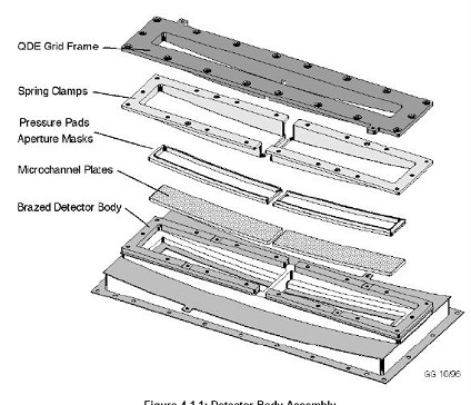
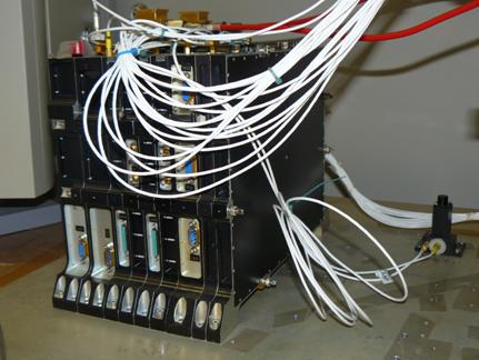
Also mounted to the backplate, but outside of the vacuum box, were two high voltage filter modules which provided the MCP, QE grid, and rear-field voltages. The backplate also supported the amplifiers, which amplified the charge collected by the anode before passing them on to the Detector Electronics Assembly. The Vacuum Assembly was thermally connected to the electronics baseplate via copper straps, which also provided chassis grounding. Figure 6‑6 shows a photograph of a Vacuum Assembly mounted in the FUSE spectrograph.
There was one Electronics Assembly for each detector; each consisted of nine interconnected electronics boxes (Figure 6‑7). The major functional components of each were:
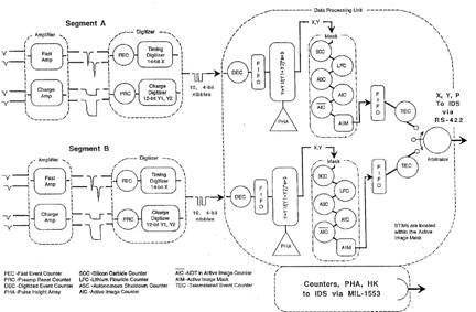
Functional block diagrams of the system are shown in Figure 6‑8 and Figure 6‑9. The following sections describe some of these components in more detail.
Figure 6‑7: Electronics Assembly and Stim Lamp Assembly of the spare detector.
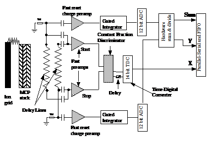
Figure 6‑8: Block diagram of the encoding electronics for the FUSE detectors.
Figure 6‑9: Functional Block Diagram of the Detector Electronics Assembly (hardware and software).
The timing digitizers determined
the X (dispersion direction) position of the charge cloud to ~20 µm by
measuring the difference in time it took the charge pulse to propagate to the
two ends of the anode, and then digitized the results to 14 bits (16384
pixels). The scale was adjusted so that the pixel size was very close to 6.0
µm, although detector distortions meant that it varied with position.
Deviations were generally only a few percent, except at the ends of each
segment, where they could be much larger. In the Y (cross-dispersion)
direction, separate Y1 and Y2 signals from the upper and lower half of each DDL
anode were digitized to 12 bits by the charge digitizers. The digitized X, Y1,
and Y2 values were then passed to the detector DPU for further processing.
Since both anode and electronics
temperatures were known to affect the measured location of photon events in the
dispersion direction, it was necessary to provide a thermal correction to the
data in the CalFUSE pipeline. Rather than relying on the measured temperatures,
however, the positions of two stimulation (‘stim’) pulses on each segment were
used for this correction. These pulses were generated by injecting charge into
the amplifiers so that pseudo-events are created near the left and right ends
of each segment, beyond the active area of the MCPs. Since the stim pulses
passed through the same electronics as incoming photons, this method provided a
more accurate method of measuring the thermal effects on the data than relying
on the temperatures. The stim pulses were normally commanded on for 59 seconds
at the beginning and end of every exposure, although for snapshot exposures
they were left on throughout the exposure. Stim rates varied slightly from
segment to segment, but were approximately 45 counts per second per stim, giving
a total rate of about 90 per second per segment. Prelaunch ground testing using
the spare detector showed that the stim pulses moved as a function of
temperature. In particular, the temperatures of the anode (best tracked via the
backplate thermistor) and the electronics (tracked with the TDC temperature)
were both shown to affect the stretch (the separation between the two stims)
and shift (position of the mean stim position) of the detector format, with the
anode temperature dominating the former, and the electronics temperature
dominating the latter. On orbit stim pulse
data show strong correlations between backplate temperature and stretch, and
between the stretch of two segments on the same detector, which is consistent
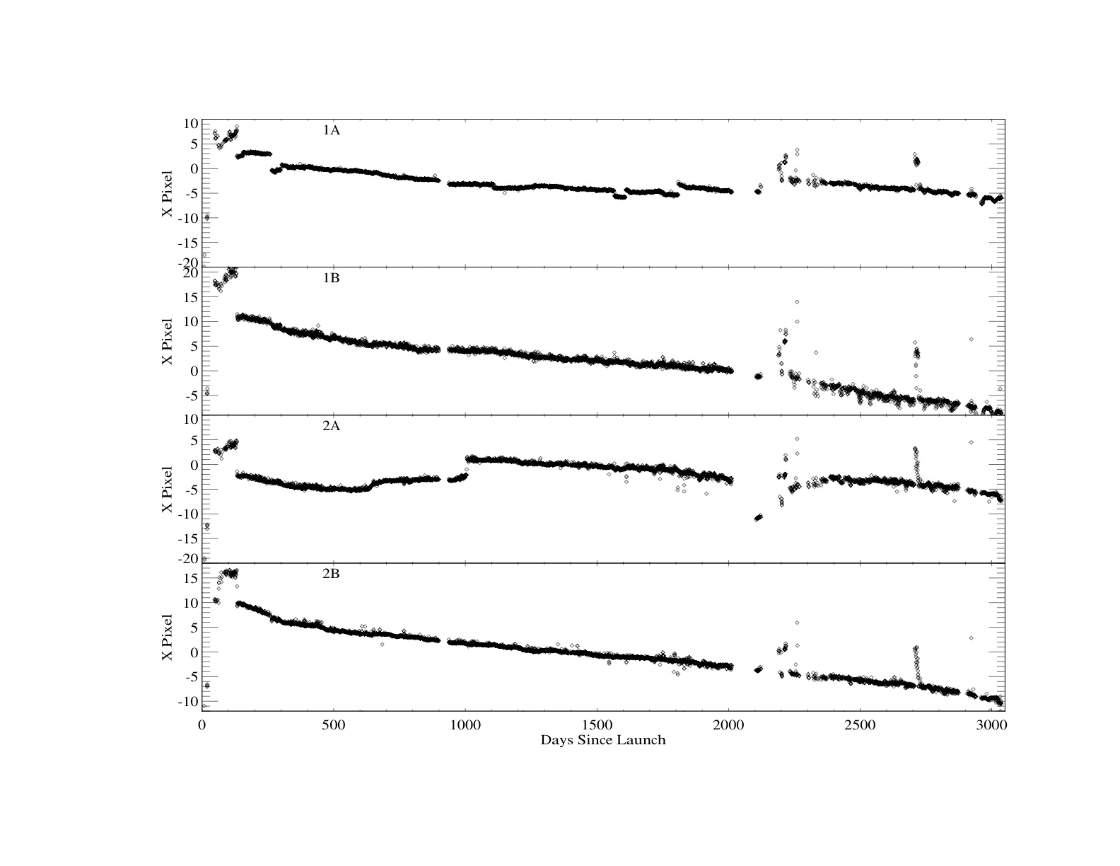
with the ground measurements. The inflight shift measurements, however, showed
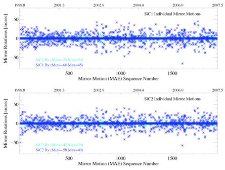
very different behavior between the segments (Figure 6‑10).
Figure 6‑10: Detector X shift, as measured by the change in position of the stim pulses, for all four
segments during the mission. Long term trends appear to dominate short term
temperature effects, particularly on segments 1B and 2B.
The positions of the stims in an
exposure are measured by CalFUSE, and a linear shift and stretch is applied to
the raw data in the dispersion direction in order to move the stims to their
nominal position. In the cross-dispersion direction only a shift is applied,
since their separation is too small to allow reliable stretch information. Because the stim pulses are
artificially generated, their shape does not exactly match the properties of
events from the MCPs. In fact, the shapes of the stim pulses change as a
function of count rate, with a sharp, single-peaked image at low count rates
turning into a double-peaked distribution at high count rates. For normal FUSE
count rates, the second peak was small and thus did not cause CalFUSE
difficulty in measuring the position. The correction for thermal
effects based on stim pulse positions assumes that the corrections are linear
over the detector, and that the thermal environment is changing slowly. Large temperature
changes, such as those due to bringing the detector high voltage from SAA level
to full, could result in rapid changes of the scale during an exposure, and
those effects are much harder to correct for. In addition, this method assumes
that the stims accurately track the overall detector format. While this is
believed to be true in general, numerous unexplained changes in stim position
that could not be correlated with any known external effects were seen (Figure 6‑10).
These may result in uncorrected errors in the calculated wavelength scale. Some
exposures are missing one or both stim pulses. In those cases, CalFUSE must
assume positions based on a record of typical positions from other exposures.
The detector Data Processing Unit
(DPU) was responsible for the electronic processing of the collected photon
events output by the digitizer. DPU memory contained two 16 KB regions from
which code could be executed; these were known as the upper core (UC) and lower
core (LC) memory regions. At boot up, a control program was loaded into memory
from an onboard EPROM. This was a basic version of the DPU code (version 16200)
which had been programmed into the PROMs before spectrograph Integration and Test
in 1997. Other versions of DPU code (Section 6.3.1.2.2.7) could then be loaded
(from the ground or IDS memory) into UC memory, and execution switched there. The main functions of the
detector Data Processing Unit (DPU) were:
6.3.1.2.1
Digitizers
6.3.1.2.1.1
Stim Pulses and Thermal Stability
6.3.1.2.2 Data Processing Unit
6.3.1.2.2.1 Overview
6.3.1.2.2.2
Calculation of Y Position
After the output from the digitizers was passed to the DPU, the Y coordinate was calculated by taking the ratio of charge between the two halves of the DDL, as Y = Y1/(Y1+Y2), where Y1 and Y2 are the charge on the upper and lower half of the delay line. This result was digitized to 10 bits (1024 pixels), although the accuracy was only ~80 µm. Y pixel sizes varied from ~ 9 to ~17 µm in the raw data, depending on detector and segment. The pulse height, or total charge collected, was also digitized at this point as part of the y calculation. The result was digitized to 7 bits and used to construct a pulse height histogram (Section 6.3.1.2.2.4).
For each segment there were four programmable masks (shown in the block diagram in Figure 6‑9) which were used to monitor the count rate in a specific region of the detector. Each mask had an associated counter which counted the number of events in each of the regions defined by the masks. The masks and counters were the Active Image Mask and Active Image Counter (AIC), the SiC and LiF masks and counters, and the Autonomous Shutdown Mask and Autonomous Shutdown Counter (ASC). The latter was also known as the SAA counter, since it was designed to measure background counts in the South Atlantic Anomaly. Each of the counters recorded the number of events that fell in a particular mask region on each segment. DPU commands were used to enable or disable regions of the segment for each counter and mask in 16 x 16 pixel regions. A complete set of aperture-specific masks for all four segments was loaded near the beginning of each observation script via the set_det_mask_f flight script. This script cleared all previous masks, then loaded an Active Image Mask that covered the entire segment, an Autonomous Shutdown Mask that fell on an unilluminated portion of the segment, and SiC and LiF masks that were placed to collect essentially all the events from the aperture specified for that observation.
The Active Image mask was used to define the region of a segment to pass to the IDS, thus acting as a spatial filter. It could have been used to exclude a region around a hot spot, for instance, so that the Science Data Bus would not be overwhelmed by these events. However, these masks were left enabled everywhere on all four segments throughout the mission. Thus, the Active Image Counter recorded the total number of events passed from the detector to the IDS on the Science Data Bus. Each event which passed through all the thresholding was output as a 32 bit word containing the detector ID (1 bit - MSB), segment ID (1), x (14), y (10), pulse height (5), and a format bit (1) to identify this as a photon event. These words were passed on to the IDS for further processing via the Science Data Bus.
The SiC and LiF masks were used to define the regions of the detector to use for target peak up, so they were different for each aperture and each segment. The objective was to determine the count rate from the object in the slit, while minimizing the count rate from the other apertures and the detector background. These masks included the entire spectral range covered on each segment, so they included any airglow in the aperture.
The Autonomous Shutdown Mask was used to monitor a region on the detector which was not illuminated by any of the apertures, so it provided a way to monitor the detector background. The DPU code used the count rate for bright object protection; if the count rate over a specified time for a particular segment exceeded a predefined threshold, the high voltage on that detector segment was lowered to SAA level. This protection was designed to minimize the chance of scrubbing the detector due to an extremely high count rate at nominal gain. As originally envisioned, this was designed in to the system primarily to protect against passing through the SAA without lowering the high voltage (as a result this counter was also known as the ‘SAA counter’). In practice, most of the shutdowns were due to event bursts, which complicated the way thresholds had to be set (Section 4.4.3.3).
The SiC, LiF, and Autonomous Shutdown masks were changed six times during the first two years of the mission (>Table 6.3‑3) in order to better align them with the position of the spectra and make them match the SIA tables (Section 6.3.3).
Table 6.3‑3: Summary of
detector mask changes during the mission An additional counter, the Fast
Event Counter (FEC – also known as the Front End Counter) measured the total
number of events over the entire segment at the output of the fast amplifiers.
The number of counts lost before the FEC, e.g. due to the MCPs themselves, is
very small at typical FUSE count rates, and was therefore ignored. The IDS code
monitored the FEC rate for each segment and shut off the high voltage for that
segment whenever the rate exceeded 45,000 counts per second for three seconds.
These values were hard coded, but IDS scripts were written to poke the relevant
memory locations in order to change them if desired. They were changed
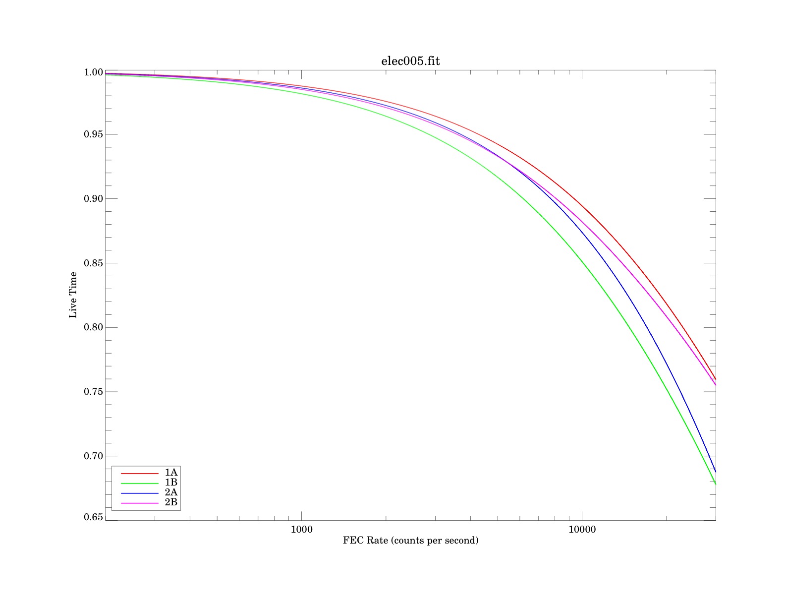
temporarily several times during the mission when bright objects were observed. The Digitized Events Counter, or
DEC, counted the number of events that were processed by the digitizer and
reached the DPU FIFO (again, over the entire segment). This was typically less
than the number of counts in the FEC, since there were electronics dead time
effects which caused events to be discarded in the digitizer. The DEC and FEC
were used in the calculation of the dead time of the instrument (Section 6.9). A summary of the masks and
counters, along with their functions is given in Table 6.3‑4.
Table 6.3‑4: Detector masks and counters
All counters were stored as
24-bit values (0 – 16,777,215) and were updated once per second. They counted
continuously from the time the detector was turned on, so they would regularly
roll over. They were typically sent to the ground via housekeeping telemetry
once every sixteen seconds, although that rate changed in certain telemetry
modes. The FEC, AIC, SiC, LiF, and ASC
counter values are saved for each exposure in the housekeeping (hskpf.fit)
files, and the first four of these are used to populate arrays in the
Intermediate Data File created by CalFUSE. The FEC, DEC, SiC, LiF, and ASC counter
values at the beginning and end of each exposure are also recorded in the
engineering snapshot and then copied into the header of the science data files.
CalFUSE uses the counter information for calculating dead time (Section 6.9)
and Y blooming (Section 4.4.7.1) effects. It should be noted that
because the SiC and LiF counters change with aperture, the count rates for
observations taken in different apertures are not directly comparable.
As described previously, a 5-bit
pulse height for each photon event is transmitted to the IDS along with the
position information. For TTAG exposures, all of this information was sent to
the ground, but for HIST exposures this pulse height information is discarded
along with the timing information. However, for both TTAGs and HISTs data, the
detector DPU also accumulated a 7-bit pulse height histogram over each detector
segment and sent it (in pieces) to the IDS. The IDS accumulated these pulse
height distributions for all four segments and downlinked a complete set of
PHDs every 128 seconds. Although these full-segment PHDs could not be used to
determine gain as a function of position, they were useful diagnostics which
could be used to monitor the gain of the detector during high count rate
observations, such as the stim lamp exposures or other HIST observations. The
higher resolution was also potentially useful for setting the onboard charge
thresholds, but they were never adjusted (except for testing) in flight.
An important function of the DPU
code was to monitor the current draw of the microchannel plates (HVIA and HVIB
for segments A and B), and the auxiliary current power supply (AUXI). The AUX
power supply was used to power the ion pumps, the detector door, and the stim
lamps. More details are given in the
discussion of High Voltage Transients in Section 6.3.5.
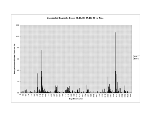
An important job of the DPU code was to continually monitor
the detector hardware and software to look for out-of-limit conditions. When a
problem was identified, a diagnostic code was issued and other protective
action was taken if warranted (Table 6.3‑5). Since the two detectors were
independent, they each issued their own diagnostic codes. Table 6.3‑5: Selected DPU Diagnostic Codes
The
diagnostic codes in the table above can be divided into three types:
Six different versions of DPU code were used during the
mission. The properties of each are summarized in Table 6.3‑6. Version 16200
was resident in the detector DPU PROM, and was loaded into lower core memory
when a detector was turned on. It was used during detector ground characterization,
spectrograph integration and test, and part of instrument and satellite
integration and test. This version had no protection for high voltage
transients (crackles). Version 16500 was provided by UC Berkeley in early 1999 to
add protection and diagnostics after the first detector crackle was seen during
instrument testing at Goddard Space Flight Center. This version also decreased
the range of upper core code memory checked by the CRC checking task. This
decreased the susceptibility to upper core SEUs by about 25%, since only 10,544
bytes (instead of 14,336) were being checked. UC Berkeley provided Version 16600 for improved crackle
protection after initial on-orbit experience. It added downlinking of the UC
CRC (in addition to the LC CRC which had been in previous versions) so that
automated code loading could be implemented. It also extended the CRC change
made in the previous version to the lower core code region. After an increase in crackles in 2001, Berkeley provided
version16603, which was functionally identical to 16600 except for an increase
in the persistence from 20 msec to 60 msec. Late in the mission, several additional versions were built
at JHU with increased persistence values. Only two of those modified versions,
16710 and 16720, were ever used during normal operations.
Table 6.3‑6:
DPU code versions used during normal operations. Different values were used during stim lamp exposures.
[1]
The threshold was set via ground command, but the values listed were rarely
changed. They were set to higher values during HV ramp ups and stim lamp
operations. [2]
Persistence values are only approximately milliseconds. [3]
Date first used on orbit. Version 16200 was resident in detector ROM and was
used for much of the pre-launch testing [4]
Date first used on orbit. Version 16500 was delivered during satellite
integration and test and was used for ground testing starting in late 1998.
The detector Stim Lamp Assemblies
(one for each detector) included the mercury vapor stimulation (or “stim”)
lamps, a mounting bracket, and a pinhole aperture to coarsely control the
amount and direction of light reaching the detectors. They were mounted to a
structural bracket in the spectrograph cavity, approximately 1.25 meters from
the detectors. Their location allowed direct, quasi-uniform illumination of
each detector, with count rates of ~2,000 to ~12,000 counts per second,
depending on segment. The stim lamps were not designed to provide a true flat
field of the detectors, but rather were included to provide general diagnostics
of detector health. Before launch, the lamps were used to provide detector
aliveness tests while the instrument was at atmospheric pressure by
illuminating the MCPs through the sapphire windows in the vacuum doors. On
orbit, they were used regularly throughout the mission as a means of monitoring
detector performance, especially gain sag (Section 4.4.2). The stim lamps were powered
through the detector auxiliary power supply, which also powered the ion pumps.
Ramping up the high voltage was a
complex process with many built in safeguards to ensure that the detector
remained safe. The ramp-up scripts: Only after all of these steps
were taken would the HV be ramped above its turn on (2500 volt) level. The
ground scripts used for ramp-up referenced a file which contained the proper
voltages. Separate scripts used for raising the high voltage for testing
purposes did not permit increases of more than 10 digital units at a time to
guard against accidentally increasing the high voltage to an unsafe level.
The detector occultation manager
was implemented during the mission in order to minimize the amount of gain sag
at the location of airglow lines. At the beginning of the mission, the high
voltage was normally left at FULL except when passing through the SAA. This
meant it was always ready for a peak-up or an observation, but it also meant
that any photons falling on the detector removed charge from the MCPs, even
though they weren't necessarily being collected by the IDS. Once the
differential gain sag problem became obvious, development began on an
occultation manager, which lowered the MCP high voltage to SAA levels whenever
it wasn't needed. This decreased the amount of unnecessary charge depletion by
removing several sources of non-productive exposure: (1) Airglow lines
illuminated the detectors during occultations and other times
between exposures, causing significant localized charge depletion.
(2) It was not uncommon
for a slew to a new target and the acquisition of that target to occur well
before an exposure began. This could be due to an intervening SAA or
occultation, for instance. The target could remain in the aperture at full high
voltage for many minutes before the exposure began. Before the implementation
of the occultation manager, this time contributed to the detector exposure and
gain sag, even though no data was collected. (3) Similarly, after an
exposure was completed, the target sometimes remained in the aperture until it
was time to slew to the next target. Before the occultation manager, this would
also add detector exposure without the benefit of collecting any additional
data. The occultation manager was used
starting on 20 November 2001, and used for the rest of the mission. It was only
turned off during times when the high voltage was being ramped up, and during
other special tests.
As described previously, the FUSE
detectors were photon-counting detectors, and the DPU produced a location and
pulse height for each detected event. These positions were passed via the
Science Data Bus to the IDS, which could either send that information on to the
spacecraft (after adding timing information) for eventual downlink to the
ground (TTAG mode), or add it to a two-dimensional image (HIST mode),
discarding the pulse height information in the process. Due to memory
limitations, an image of all four 16384 × 1024 segments couldn’t be stored in
IDS memory. Instead, only the regions around the primary spectra were saved in
memory, and they were typically binned by 8 in the cross-dispersion direction.
The primary exceptions to this procedure were the M999 stim lamp exposures,
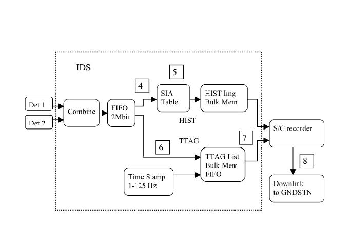
which were binned 2 × 2, and for which the entire detector area was saved. For each HIST observation, a
Spectral Image Allocation (SIA) table was used to define the detector regions
which were saved to memory. The SIA tables varied with the aperture chosen, and
they also changed during the mission as a better understanding of the location
of the spectra was gained. SIA tables were actually part of the IDS, but
because they define how the detector data is saved during histogram exposures,
they are described here. SIA tables consisted of an 8 × 64
array for each segment, with each array element referencing a 2048 × 16 pixel
region on the detector. Each array element could be set to 1 to save the data
from the associated detector region in IDS memory, or 0 to discard it. In most
cases, the observation scripts for histogram exposures called the
init_bulk_memory_f script, which loaded the standard set of SIA tables for all
apertures. A special set of SIA tables for histogram stim lamp exposures were
uploaded from the ground when needed. The standard SIA tables were changed
several times during the first few years of the mission ( Table 6.3‑7
through Table 6.3‑12). These changes were made primarily to adjust the
positions to ensure that all data from the aperture was being collected. Note
that the masks (Table 6.3‑4) were eventually set to be the same as the
SIA tables, but they did not match early in the mission. The SIA tables were downloaded to
the ground with the science data, and they are stored in the primary data unit
in the raw FITS files. Although they are not used by CalFUSE, they can be
examined to verify that the expected mask was used and was not corrupted. The
typical SIA table consists of up to 16 rectangular regions turned on, which
include, for each segment, the detector regions where the SiC and LiF spectra
fall, along with the area around each stim pulse. In many cases, one or more of
the stim pulse regions overlap with the spectral regions. The tables below
describe the regions of each detector segment covered by the SIA tables during
the mission. It is important to note that
since the SIA tables operate on the raw data coming from the detector, they are
not in the geometrically-corrected FARF, but in a distorted frame which is not
corrected for geometric distortions or thermal shifts and stretches. Thus, the
SIA table regions were oversized to avoid losing data.
Table 6.3‑7 SiC HIRS SIA Tables used during the mission
Table 6.3‑8: SiC MDRS SIA Tables used during the mission
Table 6.3‑9: SiC LWRS SIA Tables used during the mission
Table 6.3‑10: LiF HIRS SIA Tables used during the mission
Table 6.3‑11: LiF MDRS SIA Tables used during the mission
Table 6.3‑12: LiF LWRS SIA Tables used during the mission
The electronics for the two FUSE
detectors were turned on six days after launch, on June 30, 1999. On July
2, the Detector DPU code reported a change in the checksum value calculated by
its Cyclic Redundancy Check (CRC) routine. Since this CRC calculation was done
over a range of internal detector memory that contained the executing DPU code,
this meant that the code had been corrupted. The following day, a similar error
was reported on Detector 2, but neither had any apparent effect on the detector
performance. The third reported CRC error, however, caused a loss of some
Detector 1 telemetry. Only by rebooting the detector was the telemetry
restored. These errors continued to be reported at a rate of one every few days
throughout the mission. Their cause was later determined to be single event
upsets (SEUs) in the DPU memory, due to radiation from the South Atlantic
Anomaly (SAA). This susceptibility to SEUs was due to the choice of RAM in the
DPU; although the memory chip chosen had a high threshold to total radiation
dose and was immune to latchup, it had a relatively low resistance to Single
Event Effects (SEEs). Since the regions of memory being
corrupted contained the DPU code that was controlling the detectors, this was
potentially a very serious problem. Although the detector software was robust
and it was believed to be unlikely that a single bit flip could cause any
permanent damage to the detector, as a precautionary measure rules were
developed to minimize the danger. An intensive investigation was conducted to
formulate a plan for responding before the high voltage was first turned on. In
order to minimize the risk to the detector, the decision was made to only
operate the high voltage when a code image was loaded into both Lower Core (LC)
and Upper Core (UC) memory. If an SEU occurred in the active memory region, a
command was issued to jump to the alternate core on the next ground station
pass, and an uncorrupted version of the code reloaded from the ground. If the
error was in the inactive memory core, it was simply reloaded to repair it. If
both cores were found to be bad during a ground station pass, the detector was
rebooted, which shut down the high voltage on that detector. Since recovery
from a detector reboot required close to 24 hours because the ramp-up steps
were commanded from the ground, this was a major cause of inefficiency early in
the mission. In addition, the IDS flight script det_hv_f was modified to reload
several important detector parameters (SAA count rate limits, SAA integration
times, SAA HV levels, SAA reduce time, HV current limit, and AUX current limit)
after every SAA passage. This procedure was performed
manually until 8 January 2000, when version 16600 of the DPU code was loaded
onboard, along with modified IDS scripts that autonomously detected and
repaired the code. Although the code was initially loaded from IDS memory,
starting in April 2000 IDS EEPROM memory was used to free up memory for IDS
scripts. Before the autonomous code repair
was implemented, 122 SEUs had been detected on the two detectors and repaired
manually. After these changes, the autonomous correction code permitted the IDS
to identify an SEU and correct it autonomously within three minutes in most
cases. There were 1285 SEUs detected on
the two detectors during the mission. These were divided as shown in
Table 6.3‑13.
The fact that they were roughly evenly distributed between Upper Core and Lower
Core memory, and Detector 1 and 2, shows that the susceptibility was due to the
choice of parts rather than a single bad chip (note that UC and LC for a
particular detector were located on the same memory chip). No obvious
correlations of the SEU rate with time were seen, aside from changes in the
rate due to modifying the size of the memory area checked.
Table 6.3‑13: SEUs by detector and memory core.
Although most of the SEUs had no
noticeable effect on the operation of the detectors, the consequences could be
more severe when certain parts of the code were affected. In some cases, a
detector watchdog reset occurred, causing the detector to reboot. Other times
unusual behavior was seen, such as a loss or corruption of detector telemetry.
Those cases usually required rebooting the detector from the ground to recover. As expected, nearly all of the
SEUs occurred while the detector was in or near the SAA. Figure 6‑11 shows the
location of FUSE in its orbit when each SEU occurred. The figure shows that
they were concentrated near the center of the SAA, and that the spatial
distribution was similar for the two detectors. Only fifteen of the 1238 SEUs
for which the location could be identified did not fall within the SAA contour
shown. The CRC calculation took up to 40
seconds to identify a bit flip, depending on where it is in memory. In
addition, CRC values and diagnostics were reported in telemetry only once every
sixteen seconds. As a result, the times reported are likely to be somewhat
later than the actual time of the SEU, and the locations marked on the figure
will be slightly misplaced from their actual position. Figure 6‑11:
Positions of SEUs during the
mission. The dashed line shows the SAA region used by Mission Planning after 17
September 2003. No events occur below -25º due to the orbit of the satellite.
In addition to the DPU code,
detector masks (Section 6.3.1.2.2.3) were stored in the same memory chips, and
thus were also susceptible to corruption. The CRC check done by the DPU code
only checked mask memory when a mask was changed, however, so it was not
possible to tell when this occurred. As a result, there were instances early in
the mission where a mask bit was switched off due to an SEU, causing a loss of
events in that region of the detector. Once this effect was indentified, the
observation scripts were modified to reload the masks before every observation.
This greatly decreased the likelihood of this problem. During satellite-level testing,
the detector high voltage power supply current periodically had excursions that
were large enough to potentially cause damage to the detectors. To minimize the
likelihood of a detector failure on orbit due to one of these high voltage
transients, or ‘crackles’, UC Berkeley modified the DPU software to monitor the
high voltage power supply currents on segments A and B (HVIA and HVIB), and the
Auxiliary Power supply current (AUXI), at a sample rate of approximately 1
millisecond. After these modifications, whenever these currents were greater
than or equal to a threshold (a ‘mini-crackle’), a diagnostic was issued by the
detector DPU. If this threshold was exceeded for a particular length of time
(the persistence), the high voltage for both segments of the affected detector
would be turned off and an additional diagnostic issued. In addition, a portion of DPU
memory was set aside for use as a circular buffer containing the last 1024
samples (approximately 1 second) for each of these three currents, along with
three histograms that stored their distribution. The thresholds could be set via
ground command, but because the maximum current of most crackles was so high,
changing the threshold had a limited effect. The persistence, however, could
only be modified by changing the DPU code. Each change required modifying the
code followed by extensive testing. Section 6.3.1.2.2.7
describes the DPU code versions used during
the mission, along with the thresholds and persistence values for each. Figure 6‑12 shows the three
currents during a typical crackle event, as saved onboard in the circular
buffer. Although the details of each crackle event were different, the basic
features were similar in most cases: (1)
One of the currents (in this case HVIA, the high voltage current on
segment A), showed some oscillatory behavior and then went off scale. (2)
The AUX current followed a similar shape as the segment current, but had
a much lower value. Since it did not reach its maximum, it often showed the
oscillation more clearly. (3)
The current draw of the other detector segment (HVIB) was also affected. (4)
When the (HVIA) current eventually exceeded the threshold (182 in
this case) for the persistence time (60 msec), the high voltage shut down, and
the currents all dropped to zero.
Figure 6‑12: HVIA, HVIB, and AUXI during a crackle.
Table 6.3‑14 summarizes the
numbers and types of crackles and mini-crackles for each detector segment
during the mission, while Figure 6‑13 shows their distribution as a function of
time. Recall that mini-crackles had no effect on operations, while crackles
shut down the high voltage on both segments of the affected detector, which
required a high voltage ramp-up from the ground. Since the thresholds and
persistence values changed during the mission, the crackle rates at different
times cannot be compared directly, but it is clear that the incidence of
crackles is episodic, for reasons that were never understood. It is also
thought that they were more likely to occur soon after a high voltage ramp-up.
Table 6.3‑14: Number of mini-crackles and crackles
during the mission. Crackle shutdowns were the most common reason that the high
voltage on one of the detectors was not at FULL as planned during an exposure.
Since the time to return the high voltage to its nominal value after a shutdown
could be a day or longer, this was a major source of inefficiency. Plans to automate
the high voltage ramp-up process were developed, but had not been implemented
by the time the mission ended.
Similar current protection scheme
is used on the GALEX and COS detectors, but the DPU code for those detectors
provided more flexibility on setting thresholds and persistence values.
The CCD detector was a modified
version of a SITe SIA003A. This was a 1024 ´
1024 pixel thinned backside-illuminated CCD die mounted on a 2-stage
thermo-electric cooler (TEC) and sealed in a kovar package with a fused silica
window. The CCD quantum efficiency, full-well depth, charge-transfer
efficiency, dark current, and readout noise were all in accord with pre-flight
measurements. Basic characteristics of the CCD are given in
Table 2.7‑2. Half of the CCD die was masked,
so that the CCD could be operated in frame transfer mode. After a given
exposure duration, the image would be transferred rapidly to the region under
the mask and then read out slowly so that the readout noise would not affect
the accuracy of the centroid calculation. CCD thermal control was achieved
through the use of an external radiator in conjunction with a thermo-electric
cooler (TEC). The CCD package was coupled to the external radiator by means of
a heat strap fabricated from flexible copper braid that was fused at either end
into a copper block. In general, the spacecraft attitude was maintained so that
the radiator of the active FES was shaded from the sun. During in-orbit
checkout the TEC setpoint was chosen to be -32C for FES-A and -30C for FES-B.
Lower setpoints could be maintained at some attitudes, but the reduction in
dark current did not justify the operational inconvenience of tailoring the
setpoint for each attitude. With the advent of
two-wheel and one-wheel operations later in the mission, which necessitated a
much wider range of spacecraft roll angles, on-board scripts were developed
that would autonomously adjust the TEC setpoint in response to the changing
thermal environment. The resulting higher dark current and slightly-degraded
FES performance was accepted, as the pointing performance was then limited by
the torquer bars and not the FES.
The first in a series of
intermittent spontaneous FES-A reboots occurred on day 105 (April 15) of 2005.
When the reboots occurred, FES-A was left in Boot mode, and could not be
commanded to application mode without first cycling the power. In
addition, the FES would frequently not recover unless it was left powered off
for several minutes to an orbit. This led to the suspicion that some component
in the controller had an intermittent problem with heat-sinking. We attempted
to mitigate this problem by lowering the temperature of the FES-A surroundings
and by having the IDS flight scripts autonomously handle the power cycling and
rebooting sequence. We operated in this mode for several months, but
ultimately decided to switch to FES-B on July 12, 2005. FES-A was not used
for guiding during the rest of the FUSE mission. The cause of this problem was not
determined. FES-A had been subjected to survival temperatures (-5C), along with the rest of the FUSE
instrument, between Dec 28 2004, when the Roll RWA failed, and March 22, 2005,
when version T31 of the ACS software was loaded. The reboot problems began a
few weeks later. It was suspected that this prolonged cold soak had
precipitated the problem. Following the initial focusing of
the LiF2 channel for optimal spectrograph performance in IOC, the PSF of star
images in FES-B was found to be 2–3 times larger than desired (the FWHM was 4–6
pixels instead of 2 pixels), indicative of defocusing of FES-B. This
caused the light from any given star to be spread over many more pixels than
would be the case if FES-B were properly focused, reducing the contrast between
the signal and the background. Although FES had no internal
focus adjustment mechanisms, the focus could be adjusted by moving the LiF2 FPA
and/or the LiF2 primary mirror along the Z-axis (focus direction). If the
FPA was moved, the only impact to FUV data in that channel was to reduce the
throughput of the MDRS and HIRS apertures. If the LiF2 primary mirror
could also be moved, the spectral resolution of the LiF2 FUV data will be
degraded. FES-B was used successfully with these large star images during
periods when the FES-A was being annealed. When FES-B was made the permanent
guiding camera, however, the likelihood of guiding problems with faint stars
was too large. FES-B was refocused by moving the LiF2 FPA by 400 microns (See
section 6.2). The resulting image quality was
comparable to that of FES-A. The IDS was responisble for managing
FES operations, for attitude determinations based on FES data, and for
initiating slews. In essence, the IDS and FES were an integral part of an
extended attitude control system architecture. Communications between the ACS
and IDS were handled by Fine Pointing Data (FPD) packets (IDS to ACS) and ACS
status messages (ACS to IDS) transferred across the SDB. Measured quaternions,
covariances, and configuration flags were sent to the ACS once per second in
FPDs for fine pointing management. In return, the ACS provided status messages
back to the IDS. The spacecraft was responsible
for the health and safety of the satellite. Therefore the ACS was free to
reject individual FPDs or ignore the IDS altogether. The IDS did not command
the ACS, but changed the status of FPD flags to in effect request ACS
activities. The ACS monitored state changes in the FPDs and responded
accordingly. Slewing and target acquistion was
controlled by scripts executing in the IDS. The scripts controlled sequencing
of commands, while complex functions such as processing of FES images or
attitude determination were performed by the embedded guidance task software in
the IDS. Except for centroid computations performed by the FES when in
tracking mode, all fine attitude calculations were performed by the IDS.
The main steps in a basic target acquisition sequence were as follows:
More complex acquisition
procedures were needed for some observations. The main variations are described
briefly here. Offset acquisitions. In
cases where the star field in the vicinity of the target was too sparse for the
star-ID process to work, or if there were a very bright source in the FES field
of view, the first five steps of the acquisition sequence above would be
performed at an offset field. After the field was identified, the correction
slew request would include the offset needed to move directly to the desired
target position. Peak-ups. Observations
using the MDRS or HIRS apertures would include a peakup procedure folowing step
7 in the basic acquisition sequence. Peakups are described in Section 4.2.2. FES-assisted acquisitions.
In these acquisitions, the target would be left at the reference point position,
away from the apertures, and the FES would be commanded to measure its position
as well as that of the guide stars. The IDS would then compute the actual
position of the target and then command a short slew to place the target in the
proper spectrograph aperture. This mode was initially envisioned for objects
such as comets that might have poorly-known coordinates, but in practice is was
often used for routine observations. The
IDS was responsible for the operation of the instrument thermal control system
used in normal operations. Temperature data from instrument thermistors were
collected from the IPSDU, averaged, and then used to control 32 heater zone
switches in the IPSDU. Overall management was specified by a user-defined
thermal control table. The table identified which thermistors were associated
with each thermal zone and the upper and lower temperature thresholds for the
zones. Up to 4 thermistors were monitored for a zone and, when the average
temperature fell outside the zone thresholds, the heater was turned off or on.
By executing one full cycle of the algorithm every 16 seconds, the IDS
guaranteed that the temperature of each thermal zone was maintained to +/- 0.25
C of the desired temperature. Space for two tables was provided to facilitate
the loading of a new table while under thermal control of another.
The deadbands in the thermal control tables were
set at +/-0.25 C. The control system was able to maintain temperatures within
this deadband, with the exception of the equipment panels which were controlled
to within 1C, which was adequate for the electronics modules mounted on these
panels.
Under nominal three-wheel operations instrument
temperatures were well-controlled about a daily mean temperature that exhibited
no long term trends. In particular, the mirror bench temperatures on the
shaded (+X or LiF) side of the instrument exhibited no change in daily mean
temperature over the mission. During the subsequent two-wheel phase with
roll-offsets the temperatures were also, in general,
well-controlled. However, for some of the heater zones in the lower
sections of the instrument a gradual increase in the daily mean temperature was
evident - including the SiC1 mirror bench.
The behavior of the zones in the upper half of
the instrument was slightly different. This includes the spectrograph
structure, the GMA shrouds, and the gratings. Each of these zones maintained
constant or nearly constant temperatures until the pitch wheel failure in
December 2001. Following restoration of 3-axis stabilization, the mean
temperature in each of these zones was slightly (<0.1C) higher. The
temperatures of these zones exhibited a few slight mean temperature
changes/offsets later in the mission and the SiC grating temperatures increased
gradually by 0.05C over the last few years of the mission.
The LiF grating temperatures were
well-controlled. The combination of controlling the grating pie-pans in
conjunction with their thermal mass was successful in providing a stable
environment for the optics. Under normal operating conditions the grating
temperatures were controlled to within 1C. However, the grating
temperatures, in particular for the SiC temperatures, varied with solar beta
angle.
The zones within the instrument were controlled
very well throughout the mission. The slight changes that were seen were
presumably due to minor degradation of the multi-layer insulation with exposure
to solar UV radiation and atomic oxygen. The distinct step in temperatures seen
at the time of the roll wheel failure in particular may be the result of such
exposure, as this was the first time in the mission that exterior surfaces of
the instrument not covered by silver teflon blankets were exposed to the Sun
for an extended period.
The temperatures of the telescope baffles were
not controlled, as there were no functional or survival requirements to heat
the baffles. The baffle mounting to the structure was designed to decouple
mechanical stresses from differential thermal contraction of the baffles with
respect to the structure. However, the significant variations in telescope
alignment found on orbit that correlated with the Solar beta angle and orbit
pole angle, and with orbit phase, suggests that this decoupling was not
adequate. The temperatures of the door closure and unlatch HOPs, located near
the top of the baffles, are seen to vary on orbital timescales by 4-5 C on the
LiF side and by 6-8 C on the SiC side. These temperatures vary with
spacecraft attitude as well: typical variations early in the mission were 3-5 C
on the LiF side, and 12-15 C on the SiC side. Typical temperatures at the tops
of the baffles were –40 C and below on the LiF side, and –20 to -40 C on the
SiC side.
The FUSE instrument was focused
pre-flight with the provision for in-flight focus adjustments for the mirrors
and FPAs. On-orbit focus adjustments were expected due to (1) the
unavailability of a laboratory FUV source with a light beam collimated to
roughly one arcsecond accuracy and (2) the anticipated focus changes associated
with gravity release and changes in the positions of the optical elements
resulting from moisture desorption from the optical bench structure. The on-orbit instrument focus
procedure was essentially a two-step process. First, the telescope was focused
by adjusting the mirror to FPA distance for each channel. Then each
spectrograph was focused by adjusting the distance from the telescope mirror to
the spectrograph grating for each of the four instrument channels. The
FPAs were then re-adjusted to maintain the previously determined telescope
focus. The telescope focus was
determined through a series of knife-edge tests performed by scanning a target
across the edge of the FPA slit. The knife-edge test was repeated for a
set of FPA positions to determine the location along the optical axis where the
light cut-off was sharpest. Then the FPA for each channel was moved to
place the aperture at the best telescope focus as indicated by this test.
The FPA motions executed to attain the telescope focus for each channel
are presented in Table 6.6‑1.
Table 6.6‑1:
Initial in-flight telescope focus adjustments made
November 23, 1999. Adjustments
in the focus (Z) direction are limited to 10 micron increments of the
FPAs. Small residual errors account for the slight departures from
integral 10 micron changes in the adjustment values above. The true
uncertainty in the magnitude of the computed focus adjustment was at least 30
microns.
Two programs were executed to determine the
spectrograph focus. The first of these programs, I817, was executed during the
December 7 – December 9th, 1999 time interval. Multiple stellar
spectra of HD208440 were acquired through the LWRS aperture for each of 5
mirror positions stepped in 150 micron increments along the optical axis.
Data from program I817 and the
earlier knife-edge tests enabled a robust determination of the best grating to
mirror distance (the spectrograph focus) for the LiF1 and LiF2 channels.
However, the signal-to-noise of the I817 data was relatively low for the SiC
channels resulting in a less robust determination of the best spectrograph
focus position for the SiC1 and SiC2 channel mirrors. On December 12, 1999 the mirrors
and FPAs were adjusted to the best spectrograph focus for each channel based on
the data obtained December 7th-9th. LiF2, SiC1, and SiC2
previously had their FPAs adjusted to achieve the best telescope focus (mirror
to FPA distance) as determined from the knife edge testing. For these channels,
both the FPA Z position and the mirror focal distances were adjusted to focus
the spectrograph and maintain the best mirror-to-FPA distance (i.e. the
telescope focus) determined by the knife edge scans. For LiF1, the adjustment
of the mirror location for spectrograph focus matched the required adjustment
for mirror to FPA focus; hence the mirror only was moved. The FPA and mirror
position adjustments made on December 12th 1999 are presented in
Table 6.6‑2 for each channel. LiF1 SiC1 LiF2 SiC2
Table 6.6‑2: Spectrograph focus adjustments executed on December
12th, 1999 as a result of the I817 post-launch programs.
Given the low signal-to-noise of the
spectrograph focus measurements conducted as part of program I817, a second
spectrograph focus test was executed two months later as part of program I819.
The target, WD0439+466: the central star of a planetary nebula, was observed in
the LWRS slit. The spectrum exhibited many narrow molecular hydrogen lines,
which were nearly ideal for focusing. Quality data combined with careful
analysis resulted in a much better measure of the spectrograph focus. On March
16, 2000, the spectrographs were brought to their best focus position by moving
the telescope mirrors along the optical (Z) axis. The magnitude and direction
of these motions are provided in
Table 6.6‑3. These motions were generally in the opposite
direction from the first spectrograph focus adjustment, but since the data were
of significantly better quality, they were considered far more reliable.
Corresponding adjustments were made to the FPA Z positions on March 24th
2000 to maintain the mirror-to-FPA separation for LiF2, SiC1, and SiC2; the
LiF1 FPA Z position was adjusted by -100 microns (see
Table 6.2‑1 for the history of FPA Z motions).
These focus positions remained the default throughout the remainder of the
mission.
LiF1 SiC1 LiF2 SiC2
Table 6.6‑3:
Spectrograph focus adjustments executed as a result
of the I817 and I819 post-launch programs. During the
IOC shortly after launch, it was realized that the telescope mirrors underwent
periodic motions that shifted the target’s image at the telescope focal plane
and thus its spectrum in both X and Y on the detector. A source
in either of the SiC channels could move as much as 6 arcseconds in a 2
kilosecond time interval. This motion had two effects on the data: first, flux
was lost if the source drifted (partially or completely) out of the aperture;
second, the was spectrum shifted on the detector, degrading spectral resolution
for observations using the LWRS (30 arcsecond) aperture.
The procedure for the initial post-launch
channel alignment was to perform a spiral search while guiding on the target
using FES-A with LiF1 and the LWRS aperture. The FUV count rate was monitored
while using the mirror actuators to locate the target position in the three
non-guide channels. This method required use of a moderately bright FUV point
source in a fairly isolated star field to provide sufficient counts and prevent
confusion from nearby field stars. Overall, this method worked well and
was used to initially align channels to a 15-arcsecond precision.
The data were analyzed to determine the mirror
rotations required to remove the measured alignment errors at that attitude for
each of the three non-guiding channels relative to the LiF1 channel. As
further alignments and observations were attempted, it was found that all of
the channels were moving with respect to each other, with misalignments as
great as 40 arcsec.
Finer co-alignment was then performed by
stepping the roughly co-aligned images across the edge of the LWRS slits.
This method allowed for co-alignment to approximately 2 arcseconds. Early
attempts to use this method were hampered by the fact that the measurement and
adjustment were not closed loop. Scans were made and mirrors adjusted,
but no confirmation of the image position was made. FUSE would then slew
to another target, which often resulted in co-alignment being lost due to changing
the thermal environment of the instrument. Early in the mission the
source of the misalignment was unknown and the lack of a closed loop mirror
adjustment initially masked the thermal misalignment problem.
The FUSE “Image Motion” was defined as the
variation of the alignment of the SiC1, LiF2, and SiC2 channels with respect to
the reference LiF1 channel used for guiding. Although these motions were
generally quantified as being associated with the non-guiding channels, they
were caused by the motions of LiF1 in combination with the other
channels. The observed image motion was attributed to the thermal changes
induced in the instrument by changes in boresight beta angle and orbital pole
angle. The boresight beta angle is the supplement of the angle between
the satellite-sun line and the instrument line of sight and the orbital pole
angle is the angle between the orbit pole and the instrument line of sight.
To mitigate loss of data due to channel
misalignment while retaining observing efficiency, the LWRS aperture became the
primary observing aperture for most programs. For MDRS and HIRS
observations, two peakups per orbit were executed to maintain channel alignment
during an observation and obtain full spectral coverage while using these apertures.
A two-part strategy was developed to maintain
alignment of the four mirror channels. This strategy included both a
predictive component based on empirical modeling of changes in mirror position
as a function of boresight attitude and a periodic re-baselining of the
alignment.
The re-baselining component of the alignment
maintenance was achieved by performing xy-scans on a stellar target and
performing near real-time analysis to determine the direction and amplitude of
the corrective mirror motions required to attain alignment at that particular
attitude. The alignment baseline was valid for a range of beta and orbital pole
angles in the vicinity of the target. Alignment within a particular
attitude range could be maintained for approximately two weeks, assuming that
targets were scheduled within the allowed beta/pole zone. Approximately
every two weeks, xy-alignment scans were performed, the data analyzed, mirror motions
calculated and executed to remove the accumulated thermal and temporal drifts
and maintain the mirror co-alignment at the current attitude. For targets
within a beta/pole range with a different thermal environment over an orbital
period, xy-alignment scans were required to establish the mirror co-alignment
baseline at that attitude. It was also necessary to establish an
alignment baseline for every hemisphere crossing of the satellite.
Given the sensitivity of the
thermally induced mirror motions to the boresight attitude, maintaining channel
alignment by performing xy-scans for each target would have been prohibitively
inefficient. As a result, a model was generated that predicted the motion
to be executed for each mirror to maintain channel alignment for each target
observed. This predictive model was part of the planning and scheduling
process. The mirror motion scripts were uploaded to the satellite and
executed as part of the command sequence for each observation.
This predictive model for the corrective mirror
motions was derived from the analysis of xy-scans taken at multiple attitudes
in combination with the analysis of peak-up data using the 4-arcsecond wide
MDRS and the 1.25 arcsecond wide HIRS aperture. The xy-scan data provided
the magnitude and sign of the target mis-alignment in both the x and y
direction. The peak-up data provided sign and amplitude information in the
x-direction, but no y information was available. In addition to the
dependence of the mirror mis-alignment motion on spacecraft attitude, temporal
dependencies were also found but not completely nulled by the predictive
model.
Empirically, it was determined
that the secular drift of the predictive model relative to observed target
position in the different channels required obtaining xy-scans every two weeks
to re-establish the model baseline. Extreme attitude changes, such as
hemisphere crossings which were driven by the sun angle and typically resulted
in large beta changes, were not well-modeled and required xy-scans at the
target attitude to determine the appropriate mirror motions for channel
alignment. In addition, mirror motions were a strong function of attitude for
targets at large beta angles
Executing the scans, analyzing the data, and
uplinking the corrective mirror motions impacted observatory efficiency. Since
the channel misalignment resulted from thermal changes in the instrument
environment local to the mirrors, it was imperative that the mirrors were in
thermal equilibrium prior to executing the xy-scans. Thermalization
periods of 6 -12 hours were required depending upon both the beta angle and the
magnitude of change in the beta angle between targets. Analysis of scans
taken with extreme attitude changes exhibited an exponential dependence of the
target (i.e. mirror) position as a function of time, consistent with the
thermal non-equilibrium hypothesis. Achieving full positional equilibrium could
require 11 hours; however, the target was usually within the 30 arcsecond wide
LWRS aperture and monotonically approaching equilibrium within 6-8 hours.
As a result, to improve efficiency, observations were typically initiated
before completion of the full thermalization period. For time-tag
observations the data are processed by the CalFUSE pipeline as photon
lists. Signal-to-noise permitting, this facilitates the comparison of
data in temporal bins to remove secular drifts from the data.
The image motions for the two SiC channels were primarily
in the X (dispersion) direction, although small corrections in Y were
also occasionally required. For the LiF2 channel, the motion was
exclusively in Y (perpendicular to dispersion), and significantly larger than
the Y motion in the SiC channels. Y motions required corrective mirror
adjustments. In the X (dispersion) direction the FPA was used to accommodate
small changes in the predicted position of the target because FPA adjustments
were simple to implement and resulted in no loss of observatory
time. Due to the limited travel range of the FPAs, larger X motions
corrections required mirror motions to achieve co-alignment.
Analysis of the xy-scan data and
comparison of signal levels obtained in each of the channels during routine
observations enabled the formulation of a set of rules to maintain alignment
between alignment re-baselineing observations.
These predictive model
and alignment rules were incorporated into a planning spreadsheet that was
executed prior to completing the detailed scheduling of targets. The primary
alignment considerations were to restrict the changes in beta and pole angle to
within 30 degrees of the previous target. In addition, large attitude
changes required extending the observation time on a target to include the
thermalization time for that attitude and delta attitude to ensure obtaining
full spectral coverage, if needed. Hemisphere crossings and observations
at high beta angle required long thermalization times and dedicated alignment
activities. Long-term temporal dependencies were not well-modeled
necessitating the need for re-baselining alignment scans approximately
every two weeks.
Alignment activities
were required at both low and high beta angles. Motions of the LiF2
mirror at high beta angle (>90 degrees) were not well modeled an the
consequently observations requiring LiF2 data were not executed at high beta
angles without a dedicated alignment activity. Due to the paucity of data
at high beta angles, we were not able to improve the predictive model in this
regime. Pole angle was a less important consideration than beta angle for
maintaining alignment. Observations at a single beta angle for a large
range of pole angles supported this conclusion.
Later in the mission,
planning constraints necessitated by operational changes arising from failures
of the FUSE reaction wheels and associated with spacecraft safety took
precedence over alignment constraints. This periodically resulted in either
increased re-baselining activities to achieve mirror co-alignment, which was
operationally inefficient, or acceptance of limited spectral coverage as a
result of mis-aligned channels. To ensure that observations were acquired
with the necessary spectral coverage, Guest Investigators were required to specify
the channels essential for their science program. This information was
propagated through the MP database and factored into the scheduling and
detailed sequencing of observations.
Image motion was also found to have several time
dependencies. A very repeatable orbital motion was found, and was well
mapped for CVZ targets (Figure 6‑14
This source of
this motion was attributed to the thermal cycle of the orbit. For some
targets, a 24-hour period motion of as much of 8 arcsec full amplitude was
observed. This motion appeared to be roughly sinusoidal in shape. There
were also apparent long-term time dependences for some of the motions, but a
paucity of continuous data inhibited characterizing this temporal dependence.
Figure 6‑14: Orbital Dependency of Image Motion for Selected Targets
Image motion impacted FUSE science data in
several ways. (1) Channels
were misaligned for targets at beta and pole angles near the edge of the range
of nominal operations. To mitigate this, the predictor set was
continually expanded and improved. As a result, channel loss decreased
over time. (2) Re-alignment activities reduced the time available for
science data collection. Thus, realignment activities were streamlined to
use significantly less time than required early in the mission. (3) Motions of
the spectral image could result in the loss of spectral resolution, especially
for long exposures at high and low beta angles. Consequently, short
histogram exposures (<500 s) were used for bright targets. Time-tag data is
corrected for this motion in data processing
using an empirically derived correction. A
more detailed discussion is presented in the the CalFUSE pipeline paper (Dixon,
et. al 2007).
The bright limit for time-tag data was increased to allow more targets to use
this mode. (4) Tracking orbital motion for medium and high resolution
aperture observations required additional FPA motions, and impacted
efficiency.
To maintain co-alignment of the channels at the
arcsecond level required for the MDRS and HIRS apertures, an on-board peak-up
procedure was employed. This procedure slewed the telescope in small
steps to move the images across the narrow aperture. The FUV count rate
at each point was used to calculate the position of the image centroid for each
channel. Next, FUSE was slewed to the peak position for the guiding
channel. Then, each of the other three FPAs were moved to the calculated
location for each of their peak count rates. In performing this
operation, it was quickly determined that the images moved over an orbit while
pointing at a single target. Consequently, procedures were developed and implemented
to perform peakups twice per orbit to maintain alignment when using the narrow
apertures. The inclusion of mid-orbit peakups resulted in reduced observing
efficiency, but enabled full spectral coverage using the MDRS and HIRS
apertures.
As discussed in Section 4.2.3.1, the
real-time channel alignment process was time consuming. Large overheads were
incurred as a result of the time required to thermalize at the target attitude,
execute the scans, wait for ground station passes to downlink the data, perform
the scan analysis, generate the mirror motion scripts, and then uplink the
corrective mirror motions at the next available pass opportunity. This need for
ground station communications for data downlink was both a time and a
scheduling constraint. To eliminate overheads and streamline this process as
much as possible, on-board detector counter data was acquired instead of
science exposures. Figure 6‑15 depicts xy-scan counter data used to analyze an
observation. The first peak in the counts/second (occurring at between
400-100 seconds) is the y-scan; the second peak is the x-scan. The four
channels are each graphed using a different color. From inspection of the
graph, all channels are aligned in the y-direction. However for the
x-scans, the SiC data (blue peaks) are offset from the LiF1 guide channel data
indicating a misalignment of the SiC1 and SiC2 mirrors.
Figure 6‑15: xy alignment scans as depicted using the Alignment Tool Graphical Analysis. These data
are discussed in Section 6.7.4.
With the loss of reactions wheels, the pointing
jitter increased. Now, one of the primary observation scheduling constraints
was the availability of torque authority, and, in one-wheel mode, using target
sequencing to manage the spacecraft momentum. Minimizing the changes in beta
angle and pole angle between subsequent observations became a secondary
consideration. This change in planning strategy resulted in larger predictive
mirror motions and larger deviations of the mirror position from the predicted
position. As a result of the larger alignment errors and the increased
difficulty in executing maneuvers in one-wheel mode, the alignment scan pattern
was changed both in its spatial coverage and from a step and dwell pattern to a
series of continuous scans. This in turn necessitated a new alignment
assessment tool, the Channel Alignment Tool (ChAT) shown in
Figure 6‑16. In addition to
the xy-scan pattern, diagonal scans were also executed to increase the
diagnostic capability in one-wheel mode where the amplitude of pointing
excursions was much larger than previously experienced when pointing was
controlled using three reaction wheels. The erratic scan trajectories in
Figure 6‑17 and
Figure 6‑18 exemplify
the difficulty of fine-pointing with only a single wheel.
The graphical interface provided by ChAT for
interaction with the alignment scan data greatly facilitated analysis of the
scans. Regions of pointing excursions and high background were now easily
identified and excised from the alignment analysis.
Figure 6‑16: Example of Channel Alignment Tool (ChAT) Results
Figure 6‑17: (Revised) One Wheel Mode Alignment Scan Pattern
Examination of the telemetry over the eight year
lifetime of the mission never revealed an instance where the mirror motion
command only partially executed. With one exception, the infrequent
instances where the mirror motion did not appear to execute could be traced to
a manual tracking error somewhere in the alignment maintenance process.
Consequently, steps were taken to automate the procedure as much as possible.
For the first five years of the mission, LiF1
was the guide star channel and the LiF1 mirror actuators were not moved.
In 2005 due to anomalies with FES-A (see Section 4.5.3) LiF2 became the guide
star channel. The restriction on moving the LiF1 mirror was then lifted,
and LiF1, SiC1 and SiC2 mirrors were moved to align with LiF2.
There was no explicit test of the accuracy of
the mirror motions and the mirror motions were not telemetered. It could
be inferred from multiple realignments that the inaccuracies of the motions are
small compared to both the requirements and measured orbital motions.
Peakup test data showed motion accuracy about Ry for the SiC 1, LiF 2, and SiC
2 mirrors of better than 2 arcsec for small (< 6 arcsec) motions.
Moderate size motions (<30 arcsec) have been shown to have accuracies of
better than 4 arcsec. This had significant positive impact on operations after
the loss of the reaction wheels, when prioritized scheduling as a function of
spacecraft momentum management was needed. This required additional
mirror motions for a greater number of observations and hence, greater
flexibility in the mirror motion scripts.
Due to the thermally-induced relative motions of
the four telescope mirrors (LiF1, LiF2, SiC1, and SiC2) with respect to one
another (Sections 4.1.1, 6.6.1.1, and 6.7.2 - 6.7.4) the total number of mirror
motions executed was much higher than the ~900 motions per actuator that was
predicted before launch.
The
actuators were designed for 1.0 × 10⁶ motions, far more than could
reasonably be done in even a very long extended mission. As a result, although
the number of actuator motions for each mirror were tracked, there was no cause
for concern in their usage for channel alignment. Furthermore, any loss
of a single actuator on any number of mirrors is a soft failure that will cause
a minimal loss of data.
Figure 6‑20: Time series of individual mirror motions executed to maintain co-alignment of the LiF
channels.
The mirror actuators were not run over their
entire range of motion in flight. However, the defocus tests, which were
performed to assess the feasibility of executing bright target observing
programs, did move the actuators to within 20% of their full range of travel
for the LiF2, SiC1, and SiC2 mirrors. The LiF1 mirror was not defocused,
since as the guide channel at that time, the risk was not justified. No
adverse effects were noticed and the mirrors returned to their nominal in-focus
positions as commanded.
The secular drifts of the actuator
position associated with mirror co-alignment over the lifetime of the mission
is shown in Figure 6‑22
and Figure 6‑23.
The position of the actuators for each mirror, the overall repeatability of the
system, and the ability of the model to keep the mirror motions within a well
defined range is illustrated. The use of LiF2, rather than LiF1, as the guide
channel in early 2006 is evident from the plots. In April 2006, the
predictive model became less robust as is indicated in the frequent use of
larger actuator motions to obtain co-alignment.
Figure 6‑22:
The range of motion for each of the Lif1 (top) and LiF2 (bottom) mirrors
illustrating that although to co-alignment position for each actuator exhibits
a secular drift with time, this change is small and well within the range of
travel for each of the actuators.
Figure 6‑23: The range of motion for each of the SiC1 and SiC2 mirror actuators.
During IOC an investigation team was assembled
to determine the cause of the observed spectral motion. The functional form of
the motion with orbital phase was suggestive of differential thermal heating of
the instrument. A full FUSE thermal math model was correlated to the
thermal balance test data obtained during thermal vacuum test at GSFC (November
1998, January 1999) and input into a structural Finite Element Model
(FEM). This model was then used to infer temperature induced image
motions. Results of the analysis showed that, as expected, the
temperature of SiC side of the instrument and spectrograph increased as beta
angle increased. These results were in agreement with flight data
depicting the SiC mirror bench and spectrograph heater duty cycles decreasing
by 11% and 7% respectively as the instrument's exposure to the sun
increased. LiF mirror bench duty cycles were only minimally affected by
sun angle changes. SiC baffle temperatures at the upper attachment
flexure changed as much as 28 degrees Celsius when the beta angle changed from
70 to 105 degrees. The corresponding change to the LiF side was only about
1 degree Celsius. Quasi-steady-state temperature variations at these
points, caused by orbital influences, were 1 degree Celsius.
Since the spectral motion was first discovered
using airglow lines, the possible sources of the motion were isolated to the
gratings, FPAs, and detectors. Because the SiC and LiF lines incident on
a common detector behaved differently, the detector was exonorated as the cause
of the observed motions. The grating bench was eliminated as the cause of the
spectral motion because the amplitude and directionality of the spectral
motions are larger in X than in Y and it was expected that any motions caused
by the grating bencyh would be larger in Y than in X. Neither were the FPAs
regarded as a significant contributor to the spectral motion since observations
using the LWRS slit, which is much larger than the image of a typical
astronomical source, show similar motions in the spectrum of a point source and
in airglow lines that fill the slit.
The FUSE Grating Mount Assemblies (GMA) were
also investigated for any potential contribution to the in-flight spectral
motions. The existing thermal distortion analysis was reviewed for
orbital variation for the GMAs. A overview of the design was also
performed. The review of the GMAs was limited to the mount assembly since
the FUSE on-orbit performance shows no evidence that the grating glass itself
could be distorting. During the instrument design phase, a thermal model
of the GMA was constructed and coupled to the satellite model to predict an
on-orbit temperature map for the grating assembly components. That
analysis predicted that for each individual piece part of the GMA, the orbital
temperature change laterally in IPCS X and Y was negligible (< 0.02
Celsius). The orbital temperature change in the mount in the IPCS Z is
~0.2 degrees Celsius, and the worst case orbital temperature change between the
inner and outer tube temperatures is 0.2 degrees Celsius. The FEM
distortion analysis showed that translations of the center of the grating are
within short-term stability requirements.
However, the model analysis was not regarded as
conclusive given the large size of the mount and the relative flexibility of
titanium, the primary material of construction. A test simulating the on-orbit
environment was regarded as the best verification of the mount's thermal
stability.
Consequently, pre-launch tests were conducted to
determine if the gratings distorted with temperature. The gratings were
heated using their shrouds while monitoring their spectral images for
changes. The glass temperature was raised from 21 to 28 degrees Celsius
while the shroud temperature peaked at ~40 degrees Celsius. A post-launch
re-examination of this data found that the image moved 19 pixels on the
detector (~114 microns) for this temperature change in the direction of IPCS +X
for the SIC1 channel. Concurrent observations using the LiF1 channel,
without heating its shroud, exhibit only a ~3 pixel motion. These results
and the magnitudes of the motions are supported by a FEM/thermal analysis done
for FUSE by the University of Arizona.
The resulting hypothesis was that the direct
conductive path from the shroud to the grating mount hardware was heating the
"wedge" non-uniformly, possibly leading to a grating rotation.
While not conclusive, this test data illustrates the potential sensitivity of
the grating mount assembly to temperature change.
Subsequently, an on-orbit test was conducted to
test the hypothesis that the heaters may have been thermo-electrically coupled
to the spectrograph GMA.
To evaluate this hypothesis, the two grating
shrouds (LiF2 and SiC2) on the +y spectrograph axis were permitted to drift to
a lower temperature while the other two grating shrouds (LiF1 and SiC1) were
held at their nominal set point of 23 C. A temporary set point of 19 C was
chosen for the heaters. This temperature was chosen to permit acquisition of
Lyman beta airglow spectra for 2 orbits without the heaters cycling while
keeping the gratings at or above the spectrograph temperature, a contamination
related issue albeit not a severe concern after ~15 months in orbit.
Although the time required for the GMA shrouds
to reach their test thermal set-point was significantly faster than expected, a
few conclusions could be drawn. The motion of the spectrum in the dispersion
direction was not alleviated by operating with the GMA shroud heaters
off. Changing the temperature results in an offset in the zero point
position of the spectrum on the detector in the dispersion direction.
And, the functional form of the relative motion of the spectrum was the same at
the lower grating temperature as it is at the nominal temperature. The spectral
motion exhibited after the GMA shrouds were returned to their nominal
temperature was the same as it was before the temperature was lowered.
Figure 6‑24: LiF2B data over an orbital period illustrating that the spectral motion observed with the GMA shroud at 19 C
(top) is shifted/offset by ~5-6 pixels from the data acquired with the GMA
shroud at the nominal 23 C (bottom).
Figure 6‑25 Optical element layout
for LiF1, SiC1 channels. Figure 6‑26: Optical element layout for LiF2, SiC2 channels. Figure 6‑27: Optical element layout, top view. Figure 6‑28: Line drawing of an FPA mechanism, showing the two-axis stage and aperture
plate.
Figure 6‑29: Details of optics layout at detector surfaces. Figure 6‑30: Positions of optical elements. Figure 6‑31:
Side views of instrument, showing the structure, optics, baffles, electronics,
and radiators. Left: Y-Z view, Right: X-Z view. Figure 6‑32: Section views of a
primary mirror. Top: "pie-pan" enclosure, intermediate plate and
bench are shown, with positions of the actuators. Bottom: mirror dimensions and
vertex position are shown.
Figure 6‑33: Close-up view of light paths at the FPA-FES interface.
Figure 6‑34: A section view of a
grating mount assembly and grating are shown.
There were multiple effects which
caused photons that reached one of the detectors to be lost before they could
be properly recorded. We refer to these collectively as “dead time.”
Corrections for these effects, which are a function of count rate, are made in
the CalFUSE pipeline. Figure 6‑35 and Figure 6‑36
show the flow of data through the detector places in the data flow where dead time effects occur.
Information on the treatment of dead time effects by CalFUSE can be found in Dixon et al. 2007.
Figure 6‑35:
Functional block diagram showing the flow of events through the
detector electronics (1 of 2). Counts incident on the detector can be lost (1)
at the digitizer; (2) due to counts falling outside the Active Image Mask; and
(3) in the Round Robin, which combines the data from two segments on one
detector.
The following effects, numbered to match the figures, are
potential contributors to the dead time. 0 MCP response time: The first of these effects is
the response time of the MCPs themselves. If the count rate is too high in a
particular region of the plate, local gain sag may occur and subsequent
photons may not generate enough charge to be detected by the electronics. The
count rates for this to occur, however, are well above the count rates seen
during the FUSE mission, so this has a negligible effect on the data. 1 Detector Electronics Dead
Time: The inability of the detector front end electronics to process two
events that arrive within a very short time interval leads to the electronics
dead time. Analysis of the electronics design by UC Berkeley [memo reference]
showed that this effect could be characterized by the following equation:
Plive =
exp(-Rta) / (1+Rtism -x10+x6+x2-4x), X=exp(-Rtclk), where Plive = (1 –
Dead time); R is the input count rate, as given by the FEC; and ta
and t-clk and tism are constants related to the design of the Input State
Machine in the DPU ACTEL.
Analysis of science data for
each segment was used to calculate the best-fit values of ta, tclk, and tism
in the above equation so that they could be used by the pipeline. The
correction applied could then be calculated for each segment of each exposure
based on the measured FEC rate.
The parameter values in CalFUSE are given in Table 6.9-1, which were based on data obtained early in the mission. A reanalysis using all the data from the mission resulted in updated parameters, given in Table 6.9-2. The differences between th two fits are negligible for most FUSE observations, but can reach a few percent for targets at or above the bright limit. Live-time curves computed from these parameters are plotted in Figure 6-38 and Figure 6-39.
Table 6.9-1: Detector deadtime parameter values used by CalFUSE.
Table 6.9-2: Updated detector deadtime parameters
2 Active Image Mask: An Active Image Mask (Section 6.3.1.2.2.3)
which excluded part of the detector would result in a loss of counts. Since
these masks were left wide open for the entire mission, this had no effect. 3 Round Robin: The “Round Robin” combined the events
from two segments on a single detector into a single data stream for passing
to the IDS. 4 (HIST) Data Bus Limit (IDS Dead
Time): A maximum of 32,000 counts per second could be passed on the data
bus in HIST mode. If the sum of the Active Image Counter rates on all four
segments exceeded this value, CalFUSE scaled the counts appropriately. Stim
lamp exposures were the most common causes of exceeding this limit. 5 (HIST) SIA Table Screening: Use of an SIA table limits event storage to specified regions of the detector. 6 (TTAG) Data Bus Limit (IDS Dead Time): In TTAG mode, the
maximum throughput is 8,000 counts per second. 7 (TTAG) FIFO Size and Drain Rate: A 9 MB (default) region
of memory acted as a FIFO to buffer the data stream on the way to the
spacecraft recorder. Once this FIFO was full, it could be drained at only
~3500 counts per second. Thus long TTAG exposures at high count rates
had regular data droputs (Figure 6‑35). As a result, TTAG exposures were
typically limited to count rates of less than ~2500 counts per second [is
this the right number?] 8 Transmission to the Ground: Data could be lost
between the spacecraft recorder and the building of the raw data files. Figure 6‑37:
Apparent count rate as a function of time for
exposure Q11401001, which was obtained in TTAG mode, despite having a count
rate of more than 100,000 counts per second. For the first ~520 seconds the
count rates on all four segments were constant, with their sum limited to the
8,000 cps TTAG data bus limit. For the remainder of the exposure, regular data
dropouts appeared as the FIFO filled.
All of these effects have been
considered to be independent of time in CalFUSE. There were suggestions in the
data that the electronics dead time may have changed during the mission, but
the effect, if present at all, is small. Figure 6‑38: Detector live time calibration used by CalFUSE
Approximate
Date Purpose
At Launch
Prelaunch values
8/20/1999
Adjusted SiC1 and LiF1 based on first view of side
1 spectra
11/5/1999
Adjusted SiC2, LiF2 and ASC2 based on first view of
side 2 spectra
4/1/2000
Clear ASC mask before setting to avoid adding
default mask to new ASC
4/19/2000
Change ASC mask on segment 2A
11/18/2000
Reinitialize ASC mask to avoid SEUs
10/17/2001
Change size of ASC2 mask to avoid contamination
from MDRS
11/19/2001
Match masks to SIA tables
4/18/2003
Special AICs for bright objects
Mask / Counter Name
Mnemonic
Operates On
Bit in Mask Word
Description
Fast Event Counter or Front End Counter
FEC
Full segment
N/A
Total counts reaching the detector
Digitized Event Counter
DEC
Full segment
N/A
Events above threshold
Preamp Reset Counter
PRC
Full segment
N/A
Active Image Counter
AIC
Modifiable
1 (LSB)
Counts sent to the IDS
Silicon Carbide
SiC
Modifiable
2
Peakup in SiC channel
Lithium Fluoride
LIF
Modifiable
3
Peakup in LiF channel
Autonomous Shutdown Counter
ASC or SAA
Modifiable
4 (MSB)
Detector background
6.3.1.2.2.4 Pulse
Height Histograms
6.3.1.2.2.5 Current
Protection
6.3.1.2.2.6
Detector Diagnostic Codes
Diagnostic (hex)
Description
Effects on operations
16
AUXI threshold exceeded* (mini-crackle)
None
18
CRC changed in lower RAM
Associated CRC change triggers IDS process to
reload DPU code
19
CRC changed in upper RAM
Associated CRC change triggers IDS process to
reload DPU code
1A
CRC changed in ROM
None
1B
Watchdog reset as part of power up
None
20
CRC changed in segment A mask
None
21
CRC changed in segment B mask
None
22
Counts in ASC counter exceed threshold in one of
the segments (SAA shutdown)
Drop HV on affected segment to SAA level.
27
HVIA threshold exceeded (mini-crackle)
None
28
HVIB threshold exceeded (mini-crackle)
None
2A
HVIA threshold exceeded for longer than persistence
time* (crackle)
HV shut down on both segments.
2B
HVIB threshold exceeded for longer than persistence
time* (crackle)
HV shut down on both segments.
2E
AUXI threshold exceeded for longer than persistence
time* (crackle)
HV shut down on both segments.
* Not included in DPU code version 16200
6.3.1.2.2.7 DPU Code
Versions
Start Date
Code Version
Threshold[1]
(digital units) Persistence (msec)[2]
Notes
HVI
AUXI
HVIA
HVIB
AUXI
1999:181 [3]
16200
128
128
N/A
N/A
N/A
Version in DPU ROM
1999:191 [4]
16500
128
128
20
20
255
Added crackle protection
1999:334
16600
128
128
20
20
255
Downloaded UC CRC
2000:323
16600
128/182
128
20
20
255
Change to flight script
2001:326
16603
128/182
128
60
60
255
Increased persistence
2006:290
16603
182
128
60
60
255
Change to ramp up script
2006:333
16710
182
128
128
60
255
Used for detector 2 only
2007:025
16720
182
128
128
128
255
Increased persistence
6.3.1.3 Stim
Lamp Assembly
6.3.2 Normal Detector Operations
6.3.2.1 High Voltage Ramp-up
4.n.2.2 High Voltage Management:
Occultation Manager
6.3.3 SIA tables
Approximate
Start Date All
X Range 1A
Y Range 1B
Y Range 2A
Y Range 2B
Y Range Table
Names
11/20/1999
0 - 16383
160 - 319
128 - 287
288 - 399
400 - 495
siahirs1x8b
5/17/2000
0 - 16383
160 - 319
112 - 271
288 - 399
400 - 495
siahirs1x8c,
siahirs1x8d
Approximate
Start Date All
X Range 1A
Y Range 1B
Y Range 2A
Y Range 2B
Y Range Table
Names
11/12/1999
0 - 16383
288 - 447
240 - 399
208 - 319
224 - 335
siamdrs1x8b
1/13/2000
0 - 16383
288 - 447
240 - 399
208 - 319
352 - 463
siamdrs1x8c
siamdrs1x8d
Approximate
Start Date All
X Range 1A
Y Range 1B
Y Range 2A
Y Range 2B
Y Range Table
Names
10/11/1999
0 - 16383
16 - 175
0 - 175
384 - 495
480 - 591
sialwrs1x8b
3/4/2000
0 - 16383
16 - 175
0 - 175
352 - 463
448 - 559
sialwrs1x8c,
sialwrs1x8d,
sialwrs1x8e
Approximate
Start Date All
X Range 1A
Y Range 1B
Y Range 2A
Y Range 2B
Y Range Table
Names
11/20/1999
0 - 16383
624 - 783
608 - 767
544 - 655
592 - 703
siahirs1x8b
5/17/2000
0 - 16383
640 - 799
608 - 767
560 - 671
592 - 703
siahirs1x8c
3/27/2001
0 - 16383
640 - 799
592 - 767
560 - 671
592 - 703
siahirs1x8d
Approximate
Start Date All
X Range 1A
Y Range 1B
Y Range 2A
Y Range 2B
Y Range Table
Names
11/12/1999
0 - 16383
768 - 927
736 - 895
464 - 575
544 - 655
siamdrs1x8b
siamdrs1x8c
6/20/2001
0 - 16383
752 - 927
720 - 895
464 - 575
544 - 655
siamdrs1x8d
Approximate
Start Date All
X Range 1A
Y Range 1B
Y Range 2A
Y Range 2B
Y Range Table
Names
10/11/1999
0 - 16383
480 - 639
464 - 623
624 - 735
656 - 767
sialwrs1x8b
3/4/2000
0 - 16383
480 - 639
464 - 623
624 - 735
672 - 783
sialwrs1x8c
5/18/2000
0 - 16383
496 - 655
480 - 639
624 - 735
672 - 783
sialwrs1x8d
5/1/2001
0 - 16383
496 - 655
464 - 639
624 - 751
656 - 799
sialwrs1x8e
6.3.4 Single Event Upsets
Detector
Lower Core
Upper Core
1
335
271
2
299
343

6.3.5 High Voltage
Transients (Crackles)

Detector
Mini-Crackles
Crackles
HVIA (27)
HVIB (28)
AUXI (16)
HVIA (2A)
HVIB (2B)
AUXI (2E)
1
695
67
114
6
18
0
2
456
0
239
75
0
8
The values in parentheses are the diagnostic value (in hex)
issued by the detector.
6.4
Fine Error Sensor Cameras
6.4.1 FES CCD
Detector
6.4.2
Performance
and Anomalies6.4.2.1
FES-A Failure
6.4.2.2
FES-B Focusing
6.5
IDS: Instrument Data System
6.5.1 IDS–ACS
Interface
6.5.2 Observation
Sequencing and Fine Guiding
6.5.3 IDS Thermal
Control
6.5.3.1
Thermal Design
6.5.3.2
Thermal Performance
6.6
Instrument On-orbit Performance
6.6.1
Telescope
Focus6.6.1.1 Post-launch Focus Assessment
Details
FPA
FPA Motion
Z-axis
(microns)
LiF1
no change
SiC1
-99
LiF2
+48
SiC2
-81
Channel
Initial
FPA Z
Postion
(microns)FPA Z
Motions
Executed
(microns)FPA Z
Postion
Dec 12, 1999
(microns)Initial
Z Mirror
Postion
(microns)Z Mirror
Motions
Executed
(microns)Z Mirror
Postion
Dec 12, 1999
(microns)
64
0
63
293
-200
93
-100
-140
-238
-149
-150
-299
62
150
212
25
150
175
-77
none;
-150
-225
82
-150
-68
Mirror
Z Mirror Motion
(microns)
Executed
December 12, 1999
Z Mirror Motion
(microns)
Executed
March 16, 2000
Net Mirror Focus
Adjustment
(microns)
-200
No change
-200
-150
+125
-25
+150
-60
+90
-150
+250
+100
The spectrograph focus adjustments
implemented March 16th, 2000, were used for nominal operations for
the remainder of the FUSE mission.
6.7
Telescope Alignment Performance
6.7.1 Initial
Alignment
6.7.2 Mirror
Motion Anomaly
6.7.3 On-orbit Mirror
Motion Mitigation Strategy
6.7.3.1
Mirror Alignment: Baseline Maintenance
6.7.3.2
Mirror Alignment: Predictive Modeling
6.7.3.3
Channel Alignment Operations
6.7.3.4
Orbital Motion
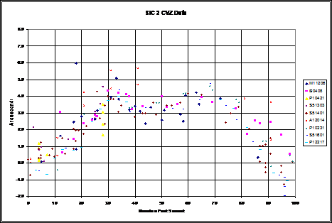
6.7.3.5
Impact and Evolution of Image Motion Corrections
6.7.3.6
Target Peak-up Strategy for MDRS and HIRS Observations
6.7.4 Channel
Alignment: Observations and Analysis
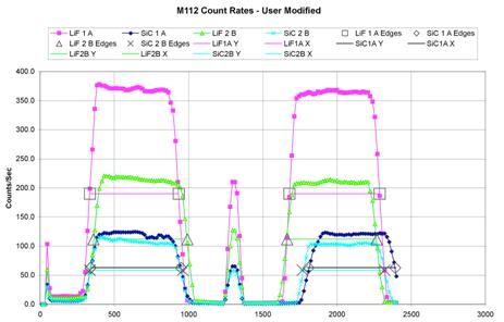
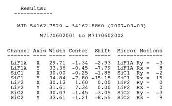
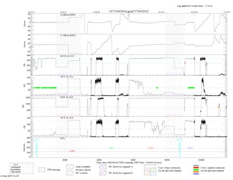
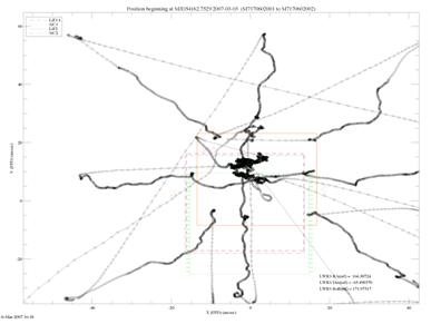
Confirmation of
the successful execution of the commanded mirror motions was inferred by one of
four methods: examination of the command sequence to verify that it had
completed properly, execution of another set of X- and Y-scans, analysis of a
follow-on peak-up activity, and/or analysis of the count rate of the next
sufficiently bright target at a comparable attitude. Depending upon the
availability of ground station contacts, addition scans or peak-ups could
require several hours or more to perform the scans and downlink the data.
Consequently, a confirmation of mirror motion execution was rarely
performed. In practice, confirmation of the count rate from the next
bright target was the primary method used to confirm that the mirrors had been
moved to their desired positions.
6.7.5 Mirror
Motion Accuracy
6.7.5.1 Mirror
Motion Tracking and Actuator Performance
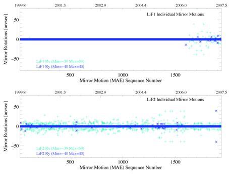
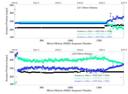
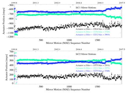
6.7.6
Spectral Motion
Anomaly: Thermal & Mechanical Analysis
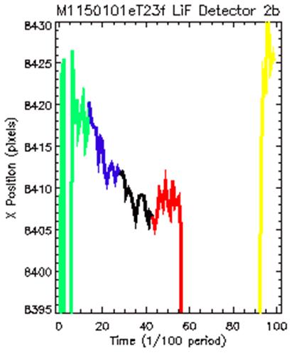
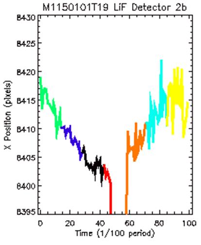
6.8
Optical Design Specifications

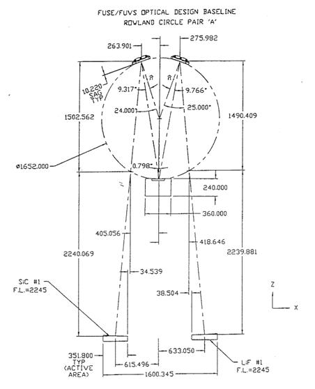
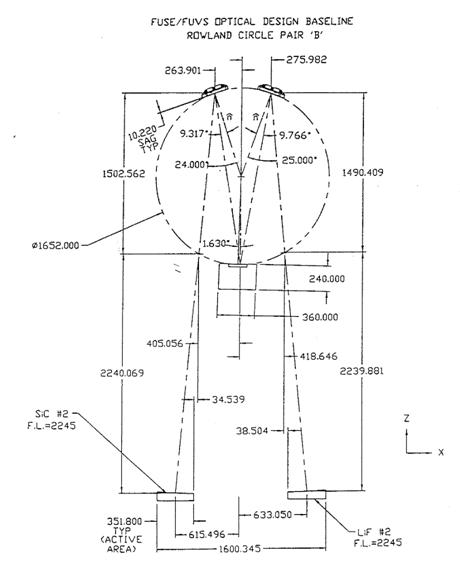
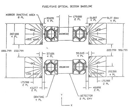
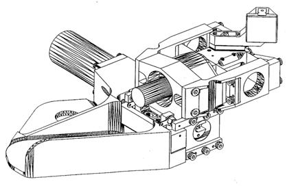
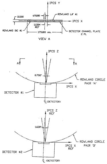

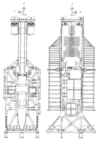
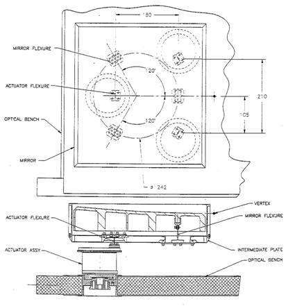
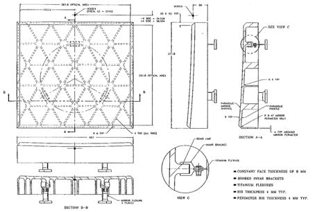
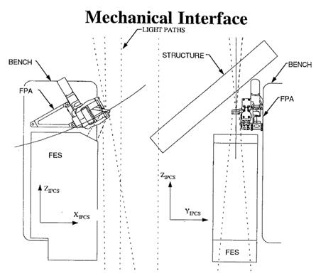

6.9
Dead Time
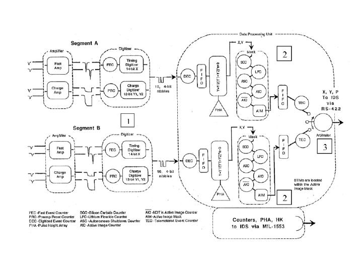
Segment
ta
tism
tclk
1A
2.76
11.68
1.50
1B
4.66
10.28
1.66
2A
5.23
8.37
1.27
2B
4.23
6.31
0.00
Segment
ta
tism
tclk
1A
5.53
9.94
2.25
1B
4.28
14.31
3.11
2A
4.85
8.89
1.08
2B
4.90
11.30
3.45