|
Step 1 -
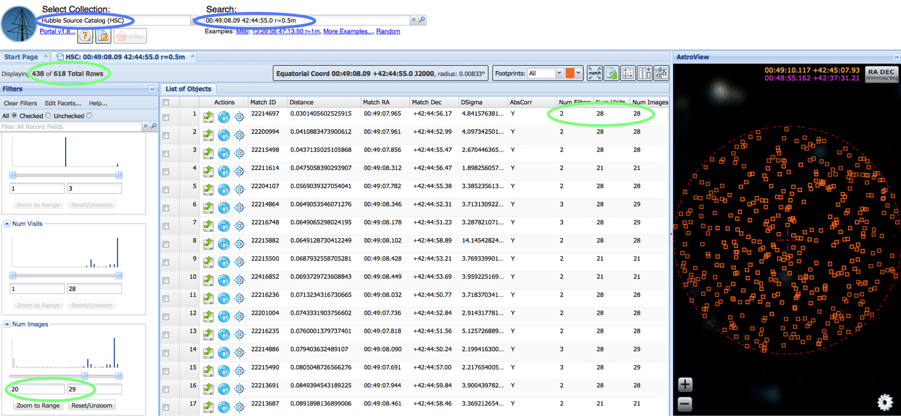
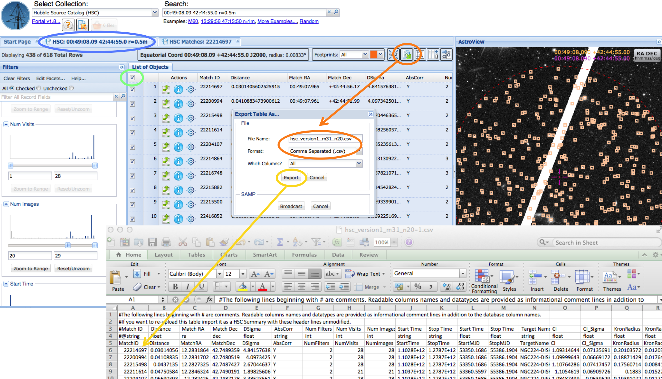
Enter the MAST Discovery Portal. Use the dropdown menu under Select Collection: (blue) to find the Hubble Source Catalog (HSC), and then enter the text " 00:49:08.09 42:44:55.0 r=0.5m " (just cut and paste if you like) into the Search box (blue). Click in the box to retrieve objects within a 0.5 minute of arc radius of the coordinates. Next, scroll down the selection Filters to find NumImages and move the slide bar to change the range to 20 to 29 (green). This controls the number of image required for a match, and can therefore be used to remove artifacts, most of which are residual cosmic rays that show up with NumImages = 1. Note that this reduces the number of objects from 618 to 438 (green), and that now all of the objects in the List of Objects have NumImages > 20 (green). |
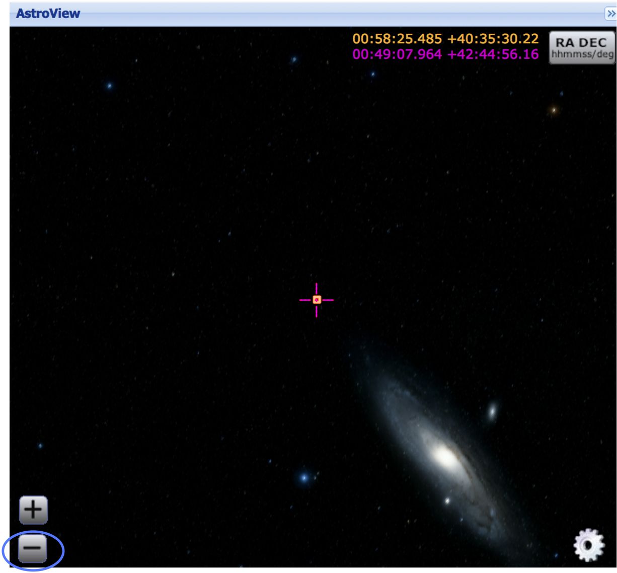
Step 2 - Play with the AstroView window. Try different kinds of images (e.g., DSS, GALAX, SDSS) by clicking the gear in the bottom right. It is also entertaining to zoom way out (blue) to see that, as implied by the Target Name in the Table View, we really are way out in the disk of M31.
|
|
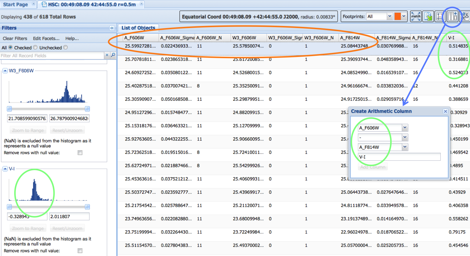 |
Step 3 - Make a new V-I colum. Click on the Create Arithmetic Column
 icon (blue) and fill in the fields to define V-I (green), which then appears as the last column in the List of Objects.
V-I will also then show up in the selection Filters field on the far left. Note the small values of Sigma for filters with repeat measurments (e.g., A_F606W_Sigma) and the relatively good agreement in the A_F606W and W3_F606W values (orange).
icon (blue) and fill in the fields to define V-I (green), which then appears as the last column in the List of Objects.
V-I will also then show up in the selection Filters field on the far left. Note the small values of Sigma for filters with repeat measurments (e.g., A_F606W_Sigma) and the relatively good agreement in the A_F606W and W3_F606W values (orange). |
|
Step 4 -
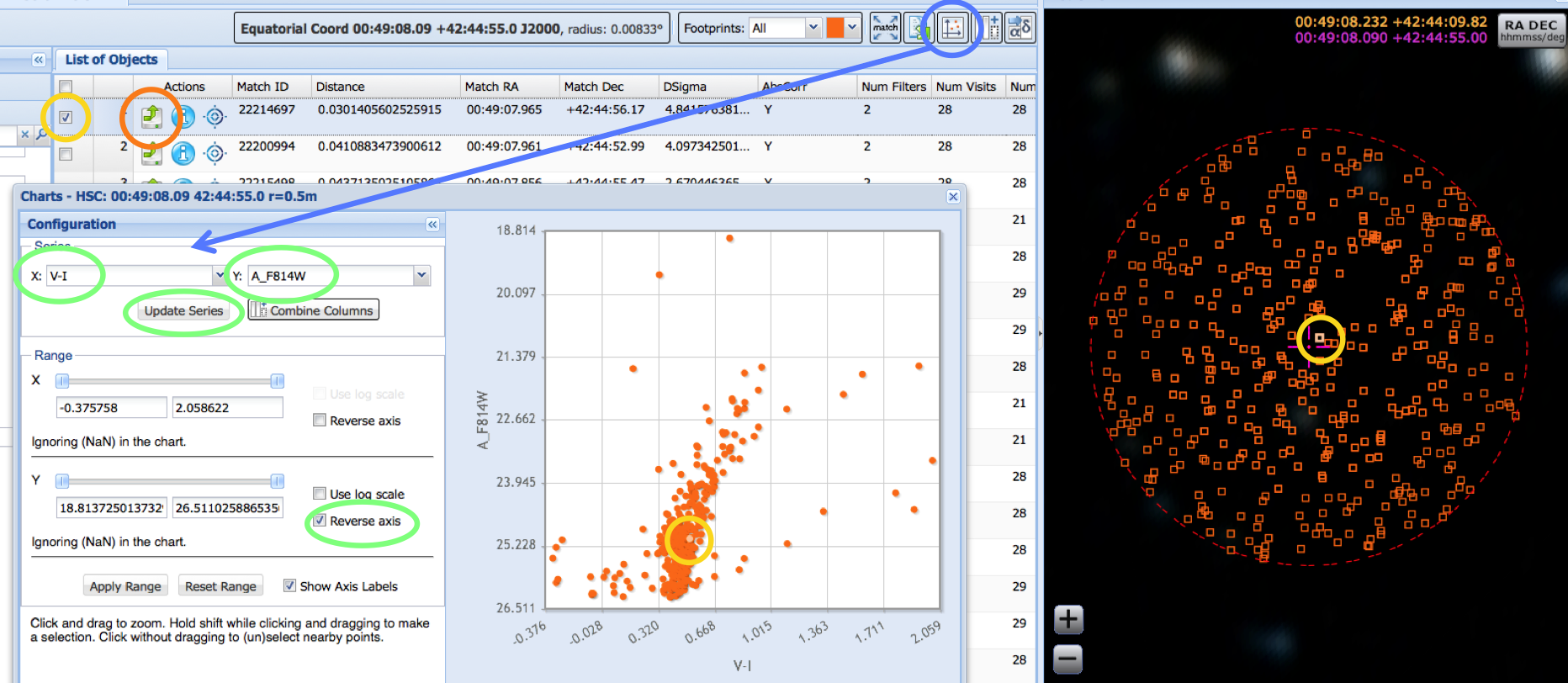
Make a V-I vs. A_F814W color-magnitude plot. Click on the View Charts for these Data
 icon (blue) and use the drop-down menu to designate the X and Y parameters (green). Then click on the Update Series button (green) to make the plot. Use the Reverse axis to flip the Y-axis.
Now click the check box in the upper left to highlight the object in List of Objects (yellow), AstroView (yellow) and in the plot. (yellow). You can instead click on a point in AstroView, or the plot, to highlight the corresponding data in the other screens as well. Finally, click on the Load Detailed Results for this Match  icon (orange) under Actions. This will bring up the HSC Detailed catalog.
|
|
Step 5 -
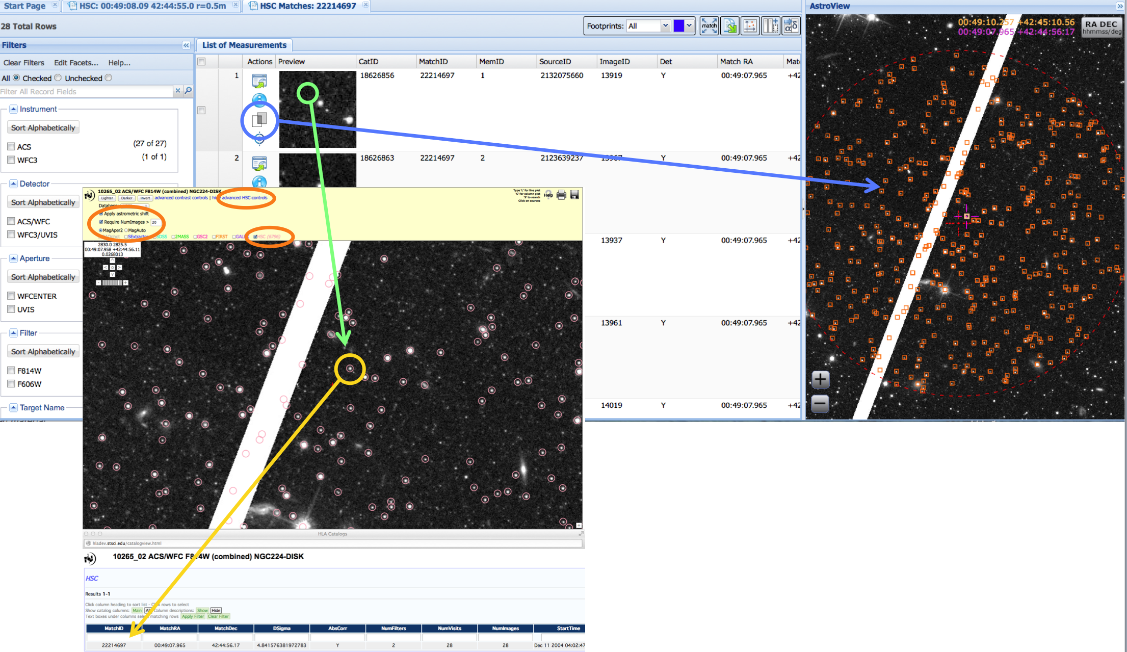
Overlay the HSC on an HLA image using Astroview, and then also using the Interactive Display. WE STRONGLY URGE USERS TO ALWAYS LOOK AT THE HSC OVERLAYED ON A HUBBLE IMAGE IN ORDER TO CHECK FOR ARTICFACTS !
First, click on the Toggle Overlay Image  icon (blue). This will bring up the image in AstroView. While you will not be able to change the contrast of the image, unlike the HLA Interactive Display, it does have the advantage of allowing you to select different subsets of the data using the selection Filters on the left.
Now click on the cutout image itself (green). This will bring up the HLA Interactive Display. Click advanced contrast controls, Apply astrometric shift, Require NumImages > 20, and then the HSC button (orange) to overlay the HSC on this particular image. Using too small a value of NumImages (e.g., > 0) can result in the inclusion of residual cosmic rays. Determining the best value for NumImages is oftern one of the most important decisions you will have when using the HSC. Click on the nearest HSC object to the center (yellow) to reveal the HSC summary form information for MatchID = 22214697. Scroll to reveal the other information for this object. The object has 28 detections with a mean A_F606W = 25.599 +/-0.022 (using 11 repeat measurements) , W3_F606W = 25.579 (no value of sigma since no repeat measurements). These are the same as what we found in Step 3. The Concentration Index (CI; difference in magnitude between 0.05 and 0.15 arcsec radius measurement) has a value CI = 1.093, which is typical for a star on the ACS. |
|
Step 6 -
Download the data for further analysis.
Return to the HSC Summary form by clicking on the appropriate page tab (blue). Then select all the data by clicking on the box in the upper left of the List of Objects (green) and then click on
the Export the Data to a Local File
 icon (orange). Fill in the File Name: (we recommend you put "version1" in the name and take a screenshot of the page for future reference), select the Format: (orange), and then click the Export button to download the table to a local file (yellow).
|
|
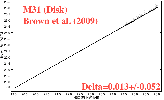
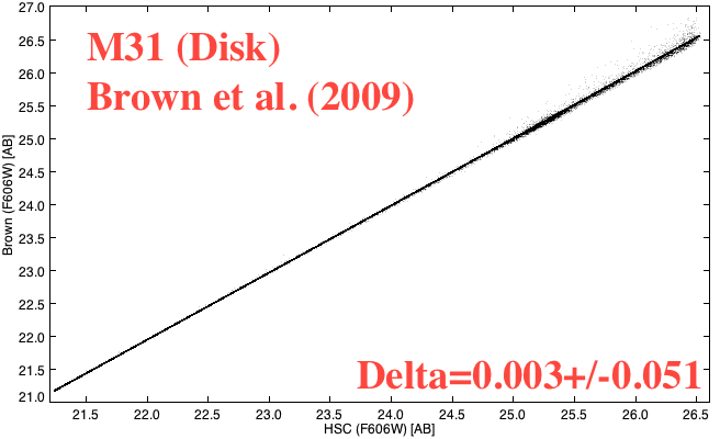
STEP 7 - Compare with the Brown et. al. (2009) photometry. If you would like to make detailed comparisons yourself you will need to download the Brown et al. (2009) catalog via the MAST High Level Science Product (HLSP)
webpage http://archive.stsci.edu/prepds/andromeda/. Below we provide a brief summary of the results; details are available in Whitmore et al. (2015).
The HSC uses the ABmag system while Brown et al. (2009) use STmag. The conversions, as provided in Brown et al (2009), are:
ABmag_F606W = STmag_F606W - 0.169 and
ABmag_F814W = STmag_F814W - 0.840
The HSC magaper2 values use an aperture with radius R = 3 pixels while Brown et al. correct to total magnitudes. To compare, we add an additional correction of 2.5log[Encircled Energy] = 2.5log[0.796] = -0.248 for F606W (similarly, -0.292 for F814W), where the values for Encircled Energy come from (Sirianni et al. 2005, Table 3.) Hence, converting from the HSC photometry system to the Brown system requires: A_606W = 25.599 (HSC Magaper2 value)
+ 0.169 (ABMAG to STMAG)
- 0.248 (aperture correction) ---------- 25.520 compared with Brown's value of 25.490 For F814W, the HSC value is 25.520 and Brown's value is 25.490. Here are plots comparing the entire dataset. See Whitmore et al. (2015) for details. |
|
STEP 8 -
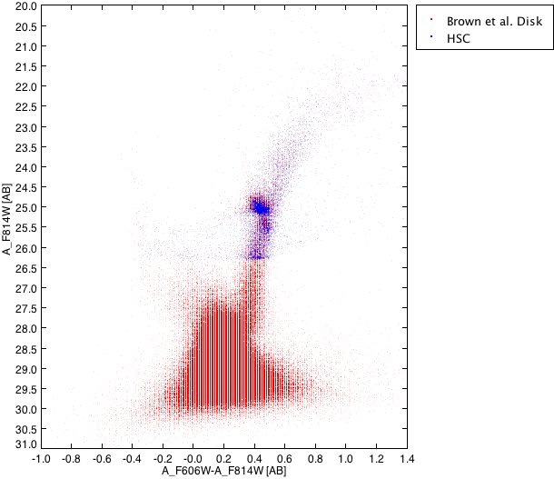
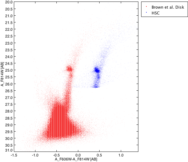
Compare the total CMD (i.e plot of F606W-F814W vs. F814W).
The following two plots show the HSC data in blue
and the Brown et al. data in red. The second figure includes an offset to
enhance the visual comparison. We note that even the fine structure in
the "red clump" (A_F814W~24.8) is very similar.
|