GOAL: This tutorial shows you how to use the MAST Discovery Portal and CasJobs to make a Color-Magnitude Diagram to search for outliers. In the process, you will learn how to download a table from CasJobs, and upload it into the Discovery Portal.
SCIENCE CASE: The science case is searching for white dwarfs (i.e. in the Globular Cluster M4; Richer et al. 1997, ApJ 484, 741).
|
Step 1 - Determine which object(s) you wish to study. Go to the Hubble Legacy Archive and input the position (blue) of your candidate object (in this case the globular cluster M4). Go to the Footprints tab (green) to see if the HST coverage is sufficient for your project. In this case, there are many imaging observations available, so this is a good object for study. |
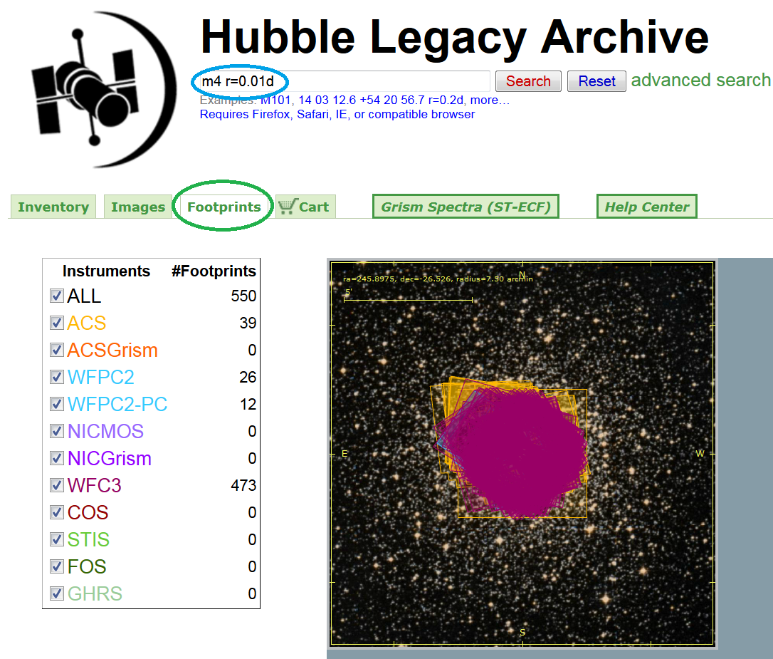 |
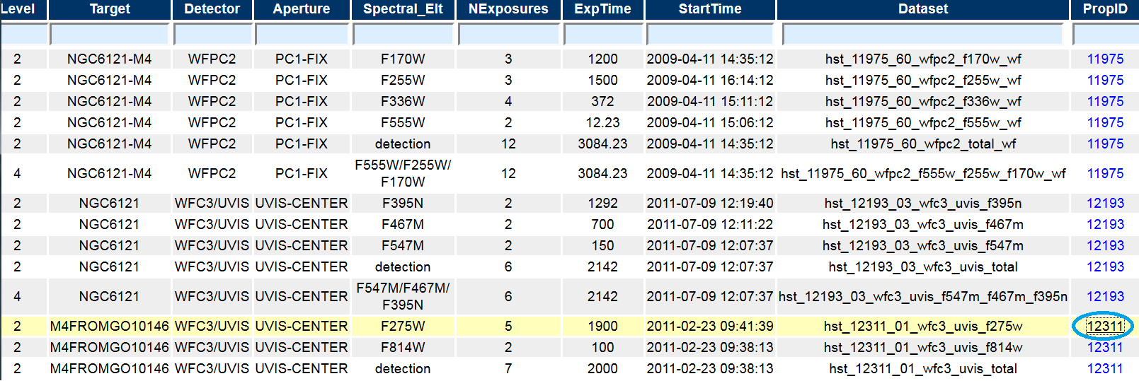
In the Inventory tab, scroll over to the PropID field and click on the ID (for example proposal 12311 (blue)). This will take you to the proposal page where you can see the abstract for the proposal, as well as papers that use this dataset.
|
Step 2 - Go to the MAST Discovery Portal.
Use the pull down menu under Select Collection to choose the
HSC (blue).
Enter (you can just cut and paste if you like) the coordinates and search
radius (i.e. 16:23:35.4 -26:31:31.9 r=200s) in the Search
box (green).
Perform the search by just
hitting a carriage return or by clicking on the
|
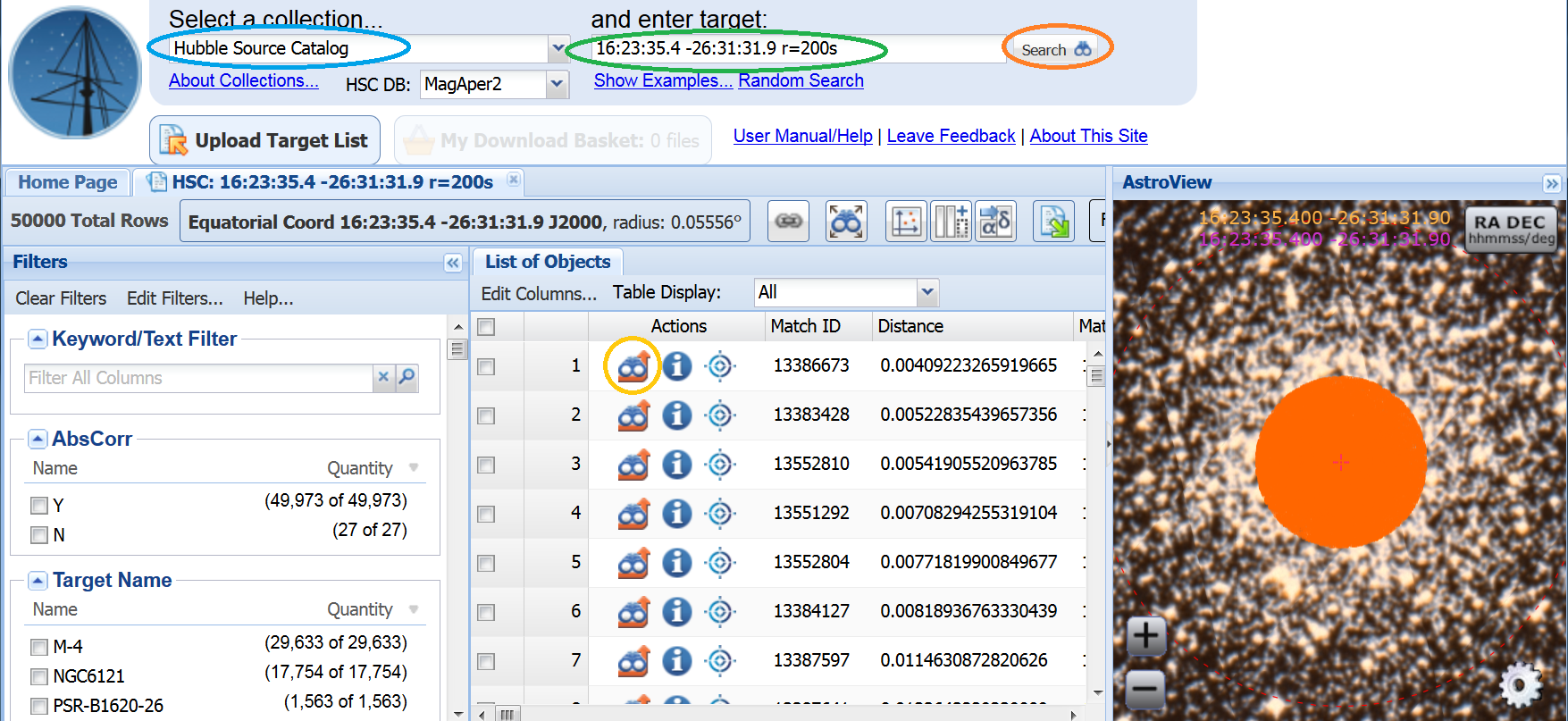 |
At this point, you may want to look directly at the HST data.
This can be done by clicking on the
 icon (yellow) under Actions,
and then clicking on the Preview image (see Use Case 1 for details).
icon (yellow) under Actions,
and then clicking on the Preview image (see Use Case 1 for details).
Note that while the HSC can be used directly for some science projects, in many cases (like this) you would need to make a much deeper catalog to get the most out of the data. In these cases the HSC provides: 1) a quick look at what data exists, 2) a feasibility study, 3) a dataset to compare with at the brighter wavelengths, and 4) the ability to link with other instruments or surveys.
|
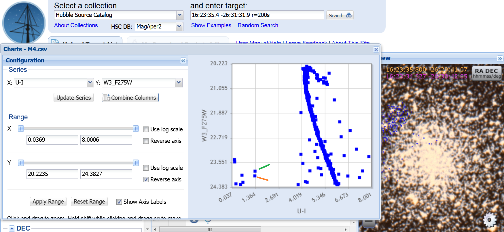
Step 3 - Make a Color-Magnitude Diagram (CMD)
Make a plot by clicking the
|
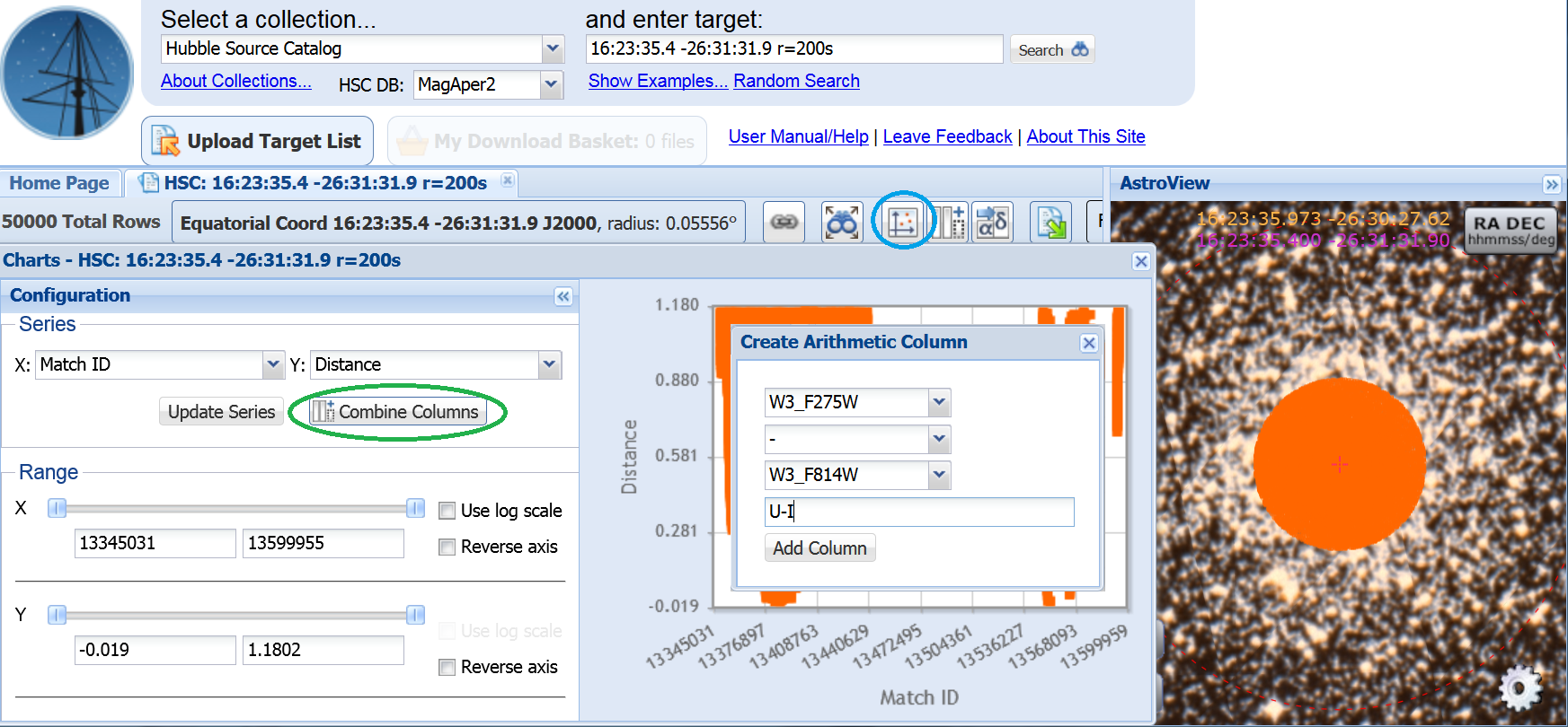 |
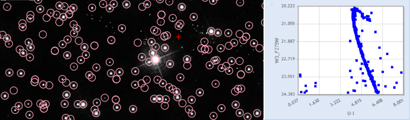
| Next, select X = U-I and Y = W3_F275W (blue). Click on the Update Series button (green) to plot the CMD. Reverse the Y axis to have magnitudes go from bright to faint (orange). The white dwarfs are blueward of the main band of stars (yellow). | 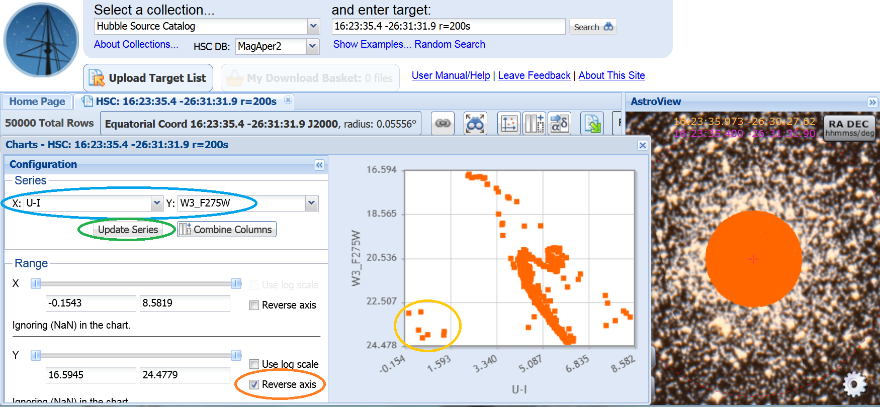 |
In some cases, you may find that there are objects in the CMD where you don't expect them. If you look at the details for these objects, you may find that they have particular high CI values (possibly due to a cosmic ray or other defect in the image) or large magnitude errors (due to the inclusion of a saturated measurement). While we attempt to screen these out when building the source lists, we are not always successful. In these cases, you should use the Filtering options to screen out the bad data.
|
Step 4 - Expand the dataset The Discovery Portal found 50,000 objects, which is currently the limit of the number of objects it will report per search. Many of these do not have F275W and F814W magnitudes, so we may be missing (many) other objects that would be of interest. Also, we have restricted our search to only 200" when ideally we would want to cover the entire cluster, which would result in even more objects that would not be reported due to the 50,000 object limit. To do a more complete search, we will use CasJobs (see Use Case 2 for more details on using CasJobs). |
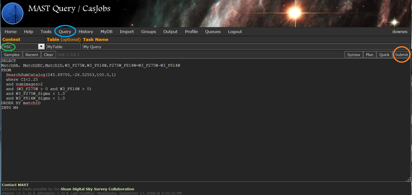 |
Enter the HSC CasJobs webpage and login. Go to the Query page (blue) and set the context to HSC (green). The query below is designed to find objects in M4 that have both WFC3 F275W and F814W magnitudes. Note that we have expanded the search radius to 500s to encompass the entire cluster, and restricted the search to exclude objects with high CI values and large magnitude errors.
SELECT
   MatchRA, MatchDEC, MatchID, W3_F275W, W3_F814W,
   F275W_F814W=W3_F275W-W3_F814W
FROM
  SearchSumCatalog(245.89750,-26.52553,500.0,1)
  where CI < 1.25
  and numimages > 2
  and (W3_F275W > 0 and W3_F814W > 0)
  and W3_F275W_Sigma < 1.0
  and W3_F814W_Sigma < 1.0
ORDER BY matchID
INTO M4
The WHERE clause defines the search parameters:
i) concentration index (CI) is less than 1.25 (to find only stars)
ii) number of images in a match (>2)
iii) W3_F275W and W3_F814W must be greater than 0 (to ignore objects with only one color)
iv) W3_F275W_Sigma and W3_F814W_Sigma must be less than 1.0 (to ignore objects with poor measurements)
Submit (orange) the query for processing.
|
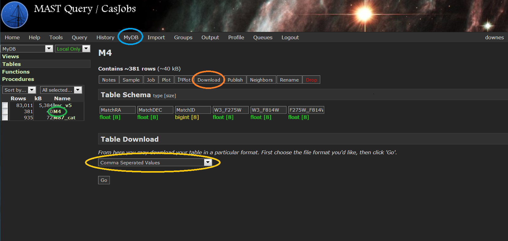
Step 5 - Export the CasJobs data
After the query has finished, go to the MyDB (blue) page. Find the dataset (M4) in the list on the left and select it (green). Note that there are ~381 objects. We need to download the data so we can import it into the Discovery Portal for plotting. Select the Download option (orange). Select your format (yellow) and click on Go. |
 |
| After hitting Go, you are taken to the Output page. Once the dataset is available, click on Download (blue). | 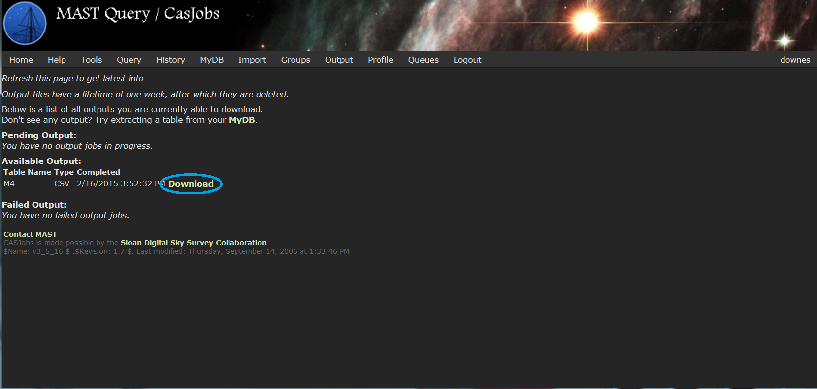 |
|
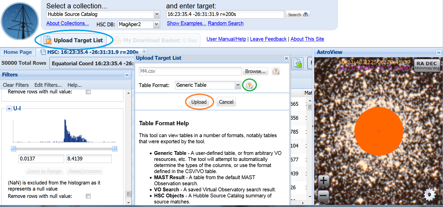
Step 6 - Import the catalog into the Discovery Portal
Prior to ingesting the catalog into the Discovery Portal,
you must change the name of the MatchRA column to
RA and the MatchDEC column to DEC; you can also rename
the F275W-F814W column to U-I.
Then go to the
Discovery Portal and click on the
|
 |
After importing, you will see the catalog and the objects overlaid on the DSS image.
|
Step 7 - Make the Color-Magnitude Diagram
As we did in Step 3, make the plot by clicking the
|
 |
|
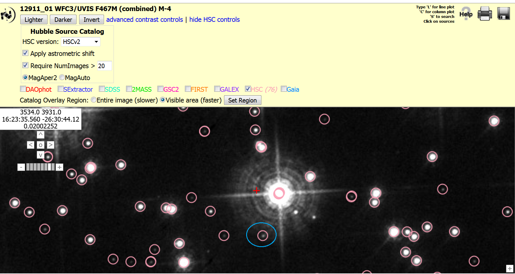
The white dwarfs are blueward of the main band of stars. Of the 8 objects in the WD area, 6 are in Richer, 1 is not in the WFPC2 FOV (green) used by Richer and hence is a new white dwarf candidate, and 1 is not visible on the WFPC2 F814W image (but is in the WFC3 data so is in the HSC; orange). It is always a good idea to go back to the HLA and look at each object to make certain it is not an artifact or have other issues. Below is a blowup of the one candidate (blue) that was not visible on the original WFPC2 F814W image. |
 |
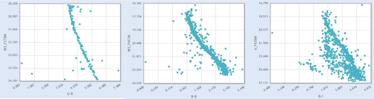
With the techniques above, it is easy to make other Color-Magnitude diagrams.
 icon (
 icon
(
icon
( icon (
 icon (