GOAL: Determine whether the HSC Version 2 astrometry is accurate enough for measuring positions for a NIRSpec MOS observation. The astrometric accuracy needs to be better than about 15-25 mas for optimal target acquisition accuracy (see NIRSpec MPT: Catalogs for details). In many cases NIRCam images must be taken with JWST to provide this level of accuracy, but in certain cases where HST observations have been taken it may be possible to use the HSC to provide the target lists, and hence save JWST observing time.
NOTE: While the example here is for NIRSpec MOS observations, the steps provided here can be used to determine if the HSC astrometry is sufficient to support other types of JWST observations (e.g. NIRSpec target acquisition, MIRI Medium Resolution Spectroscopy).
SCIENCE CASE: Provide a target list of star cluster candidates in a region in the north-cental part of M51 with better than ~20 mas astrometric accuracy. In order to do this, we must confirm the folowing:
|
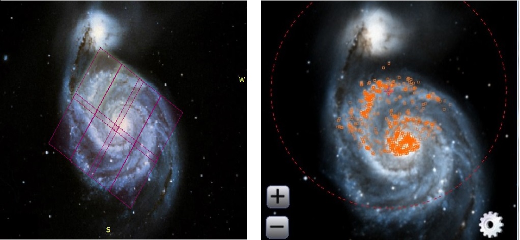
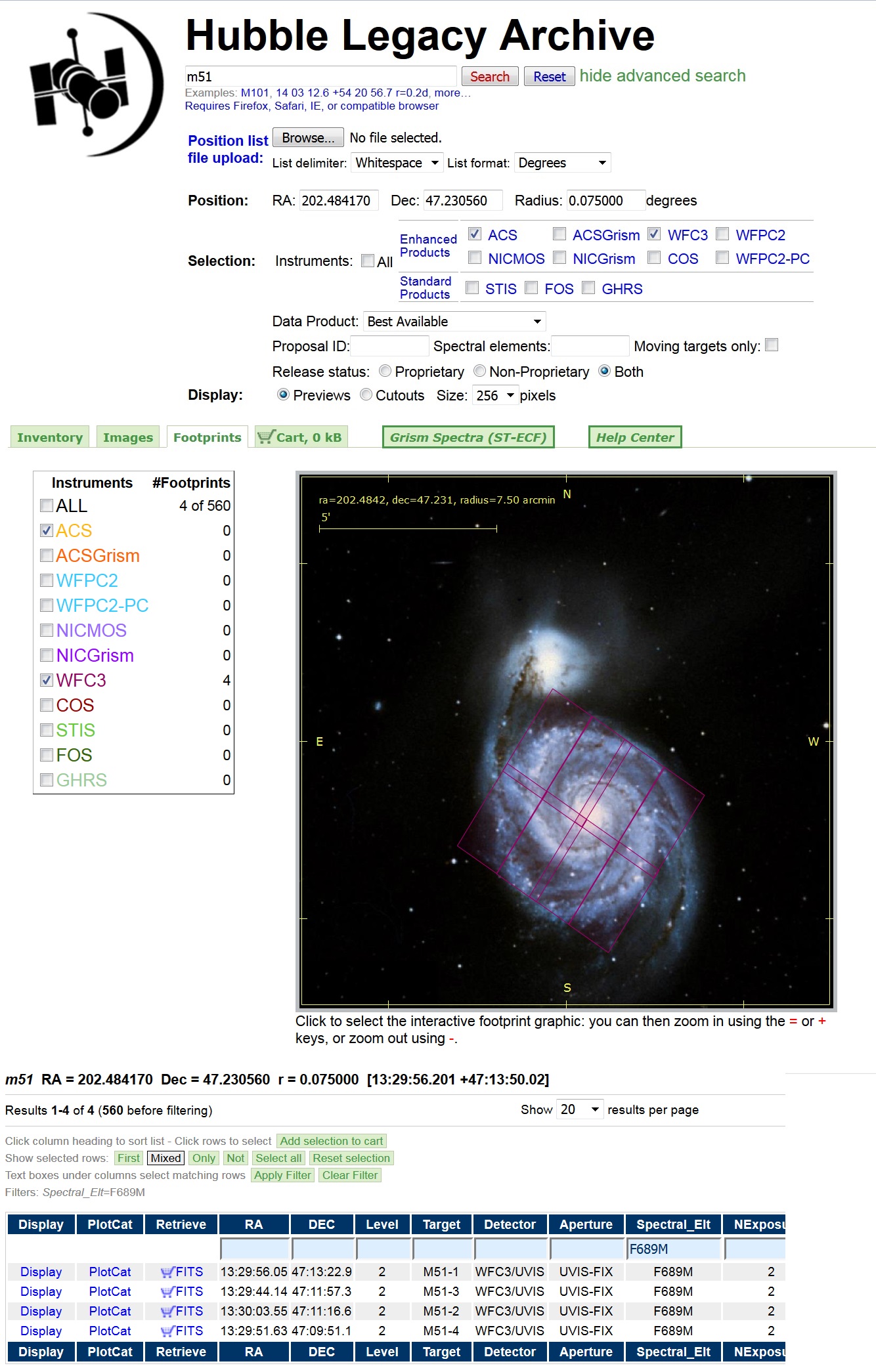
Step 1 - Determine what instrument/filter has the science targets. Use the Hubble Legacy Archive (HLA) to search the ACS and WFC3/UVIS images (i.e. the only instruments with sufficient spatial resolution for our purposes). You will find a wide range of potential instrument/filter combinations, but some will not be suitable for our purposes (e.g., the Nexposure = 1 visit-based ACS images used to make the famous mosaics are not included in the HSC since they have cosmic rays). In this exercise we will use the WFC3/UVIS F689M to overlay the HSC, which gives good coverage of the galaxy. |
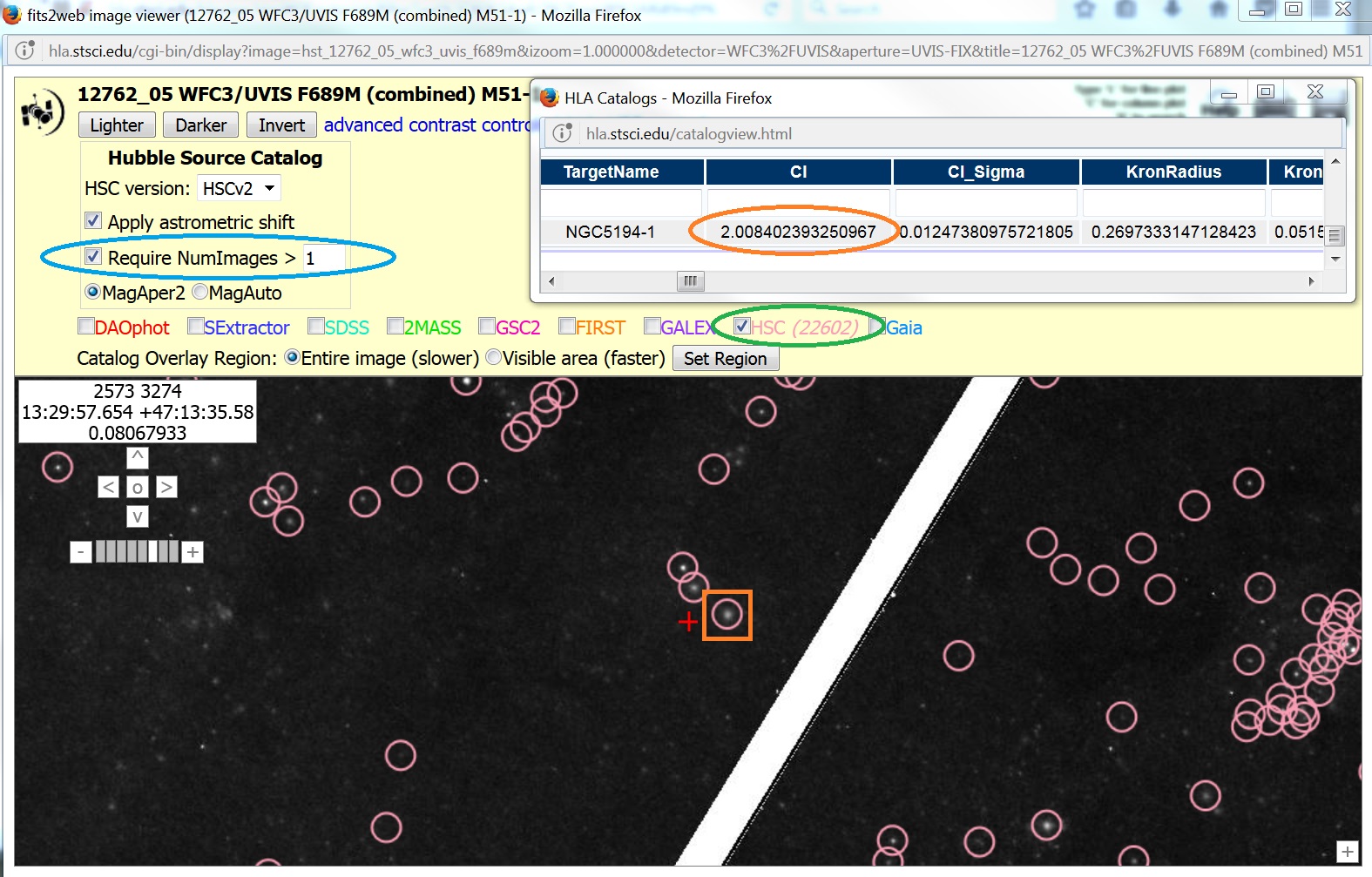
Bring up the interactive display, set Require NumImages > 1 (blue), and overlay the HSC catalog (green). Examine the image and see that there are extended sources (e.g. Concentration Index >> 1) that are cluster candidates (orange).
|
Step 2 - Go to the MAST Discovery Portal.
Select HSCv2 from the pull down
menu (blue) in the upper left, enter M51 as
the target and click on the Search
|

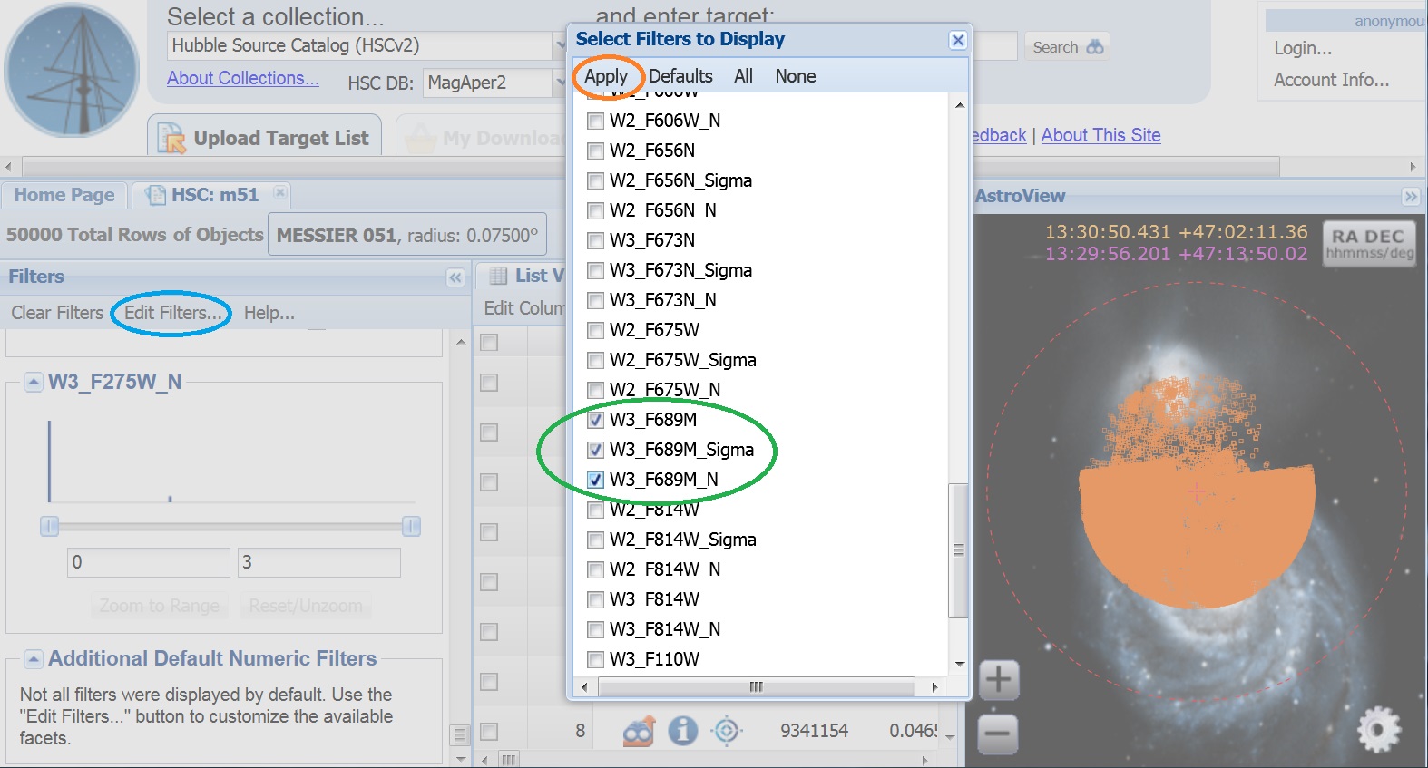
The default number of selection filters only includes down to the F275W filter. Click on the "Edit Filters" (blue), select the W3_F689M filter (green), and hit "Apply" (orange).
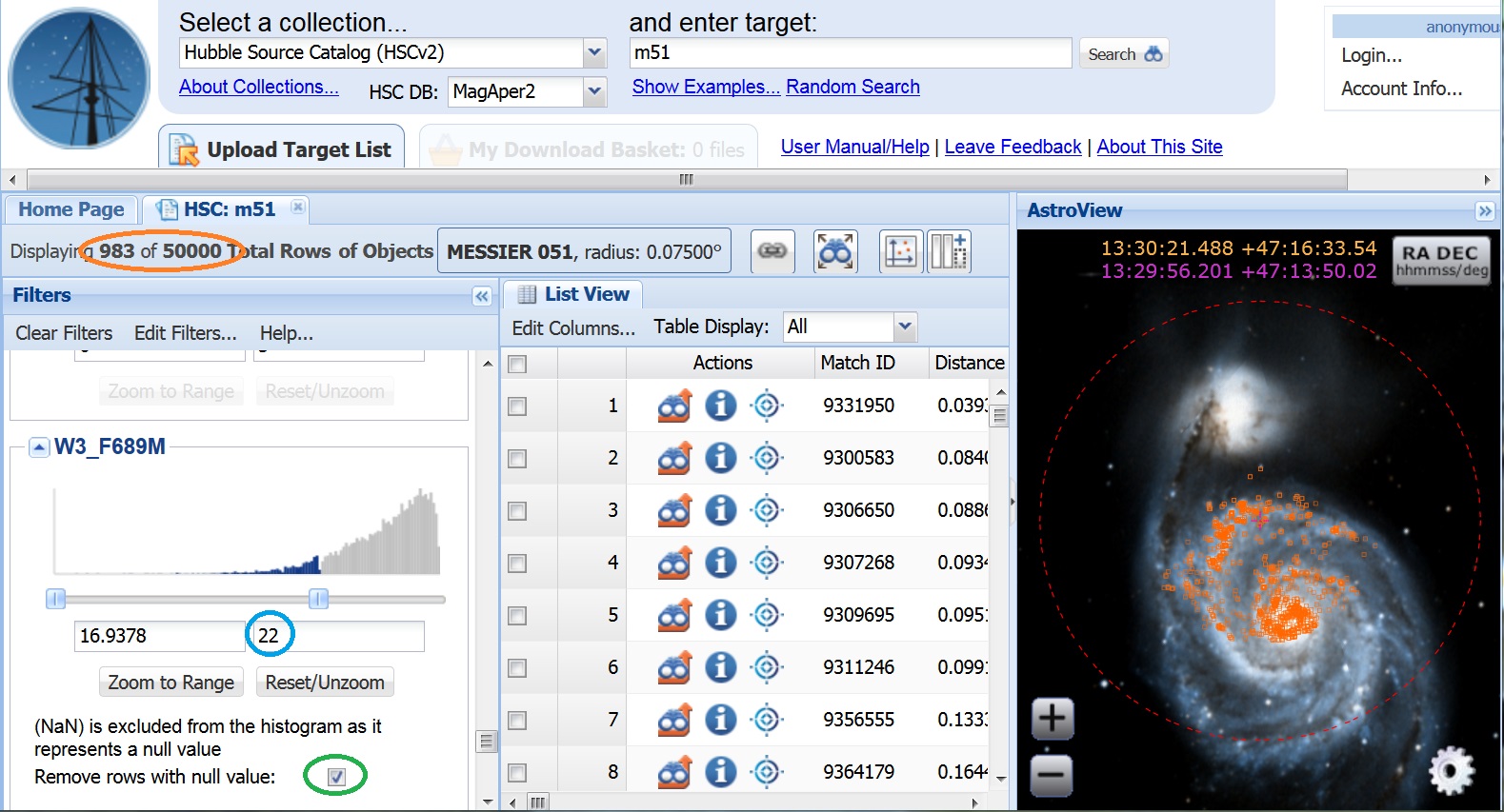
Now select only the WFC3_F689M objects brighter than 22 (blue), and click the "Remove rows with null value" box (green) just below W3_F689M histogram. This will reduce the number of objects to 983 (orange), making the cross matching with the GAIA catalogs (which will be the reference frame for JWST observations) much faster.
|
Step 3 - Overlay on an HLA image.
The DSS image used for astroview does not have the
spatial resolution
needed to see the sources very well. Click on the "Load Detailed
Results for this Match"
|
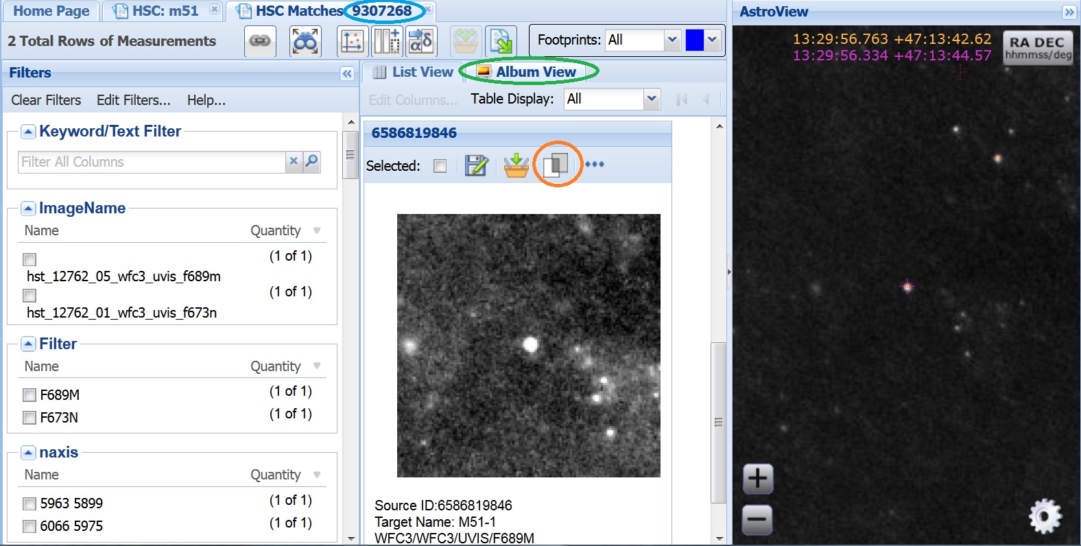
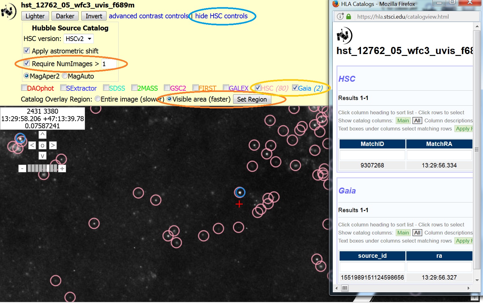
We selected this object to center on since it turns out to be a GAIA source. Our goal is to determine how good both the relative and absolute astrometry are for the HSC in this field. We will assume that GAIA represents the "truth" value. Hence we need HSC stars that are also found in the GAIA catalog to perform the analysis. To verify that the HSC object is also in GAIA, click on the cutout image to bring up the HLA interactive display. Open up the HSC controls (blue), select "Require NumImages" to be >1 (green), set the Catalog Overlay Region to be "Visible area" and click on "Set Region" (orange), and select the HSC and GAIA catalogs (yellow). We can now verify that the object is in both catalogs.
|
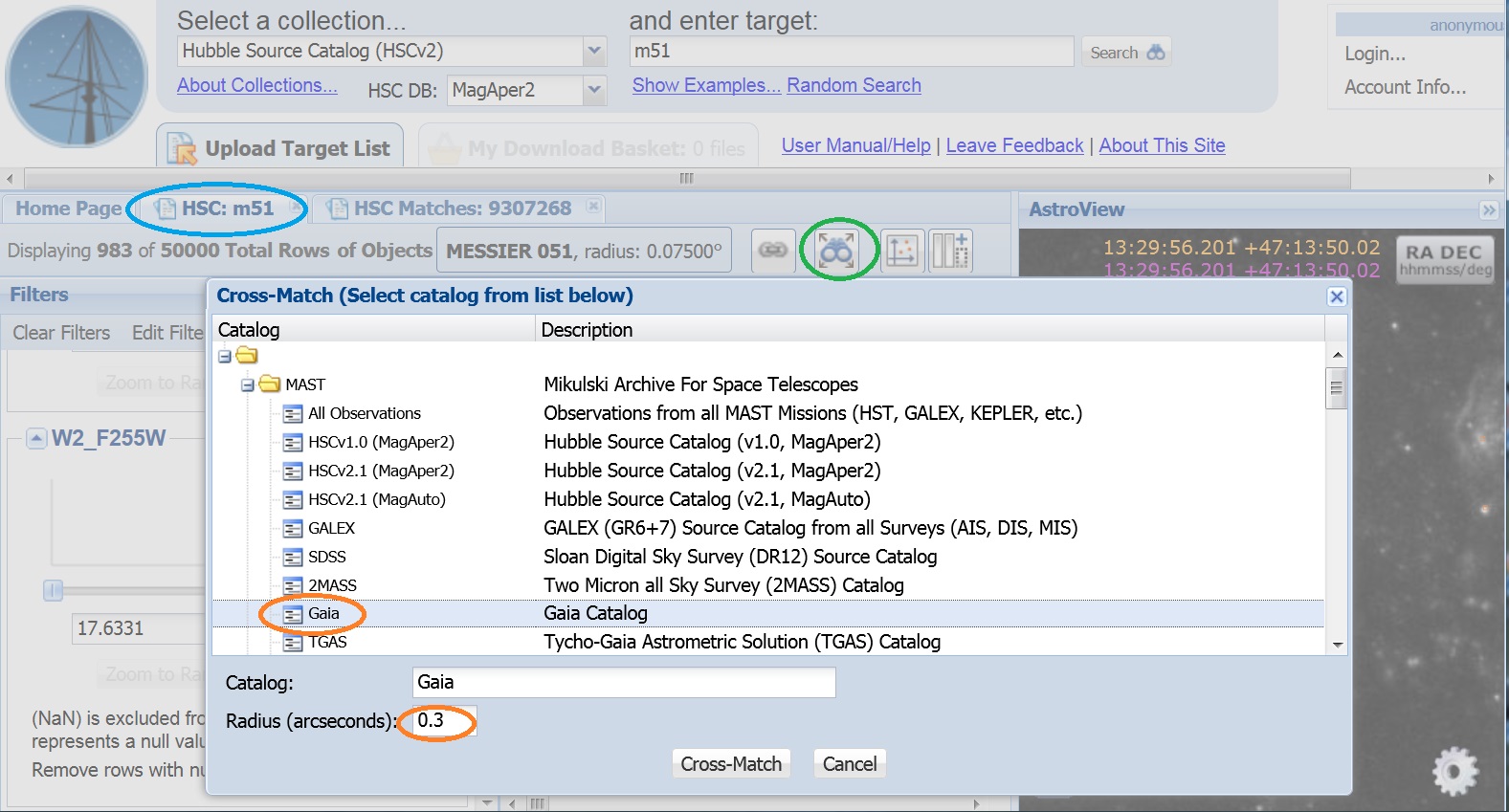
Step 4 - Cross match with GAIA. This will allow us to determine whether the HSC accuracy is sufficient for our purposes, and will also provide any positional offsets required to align the HSC with GAIA more precisely.
First, click back on the HSC:M51 home page
(blue)
to get to the full catalog,
and then click on "Cross Match this table with other Catalogs"
|
|
Step 5 - Determine the Delta-RA and Delta-Dec values and make a plot.
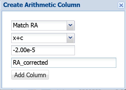
Use the "Create Arithmetric Column" |
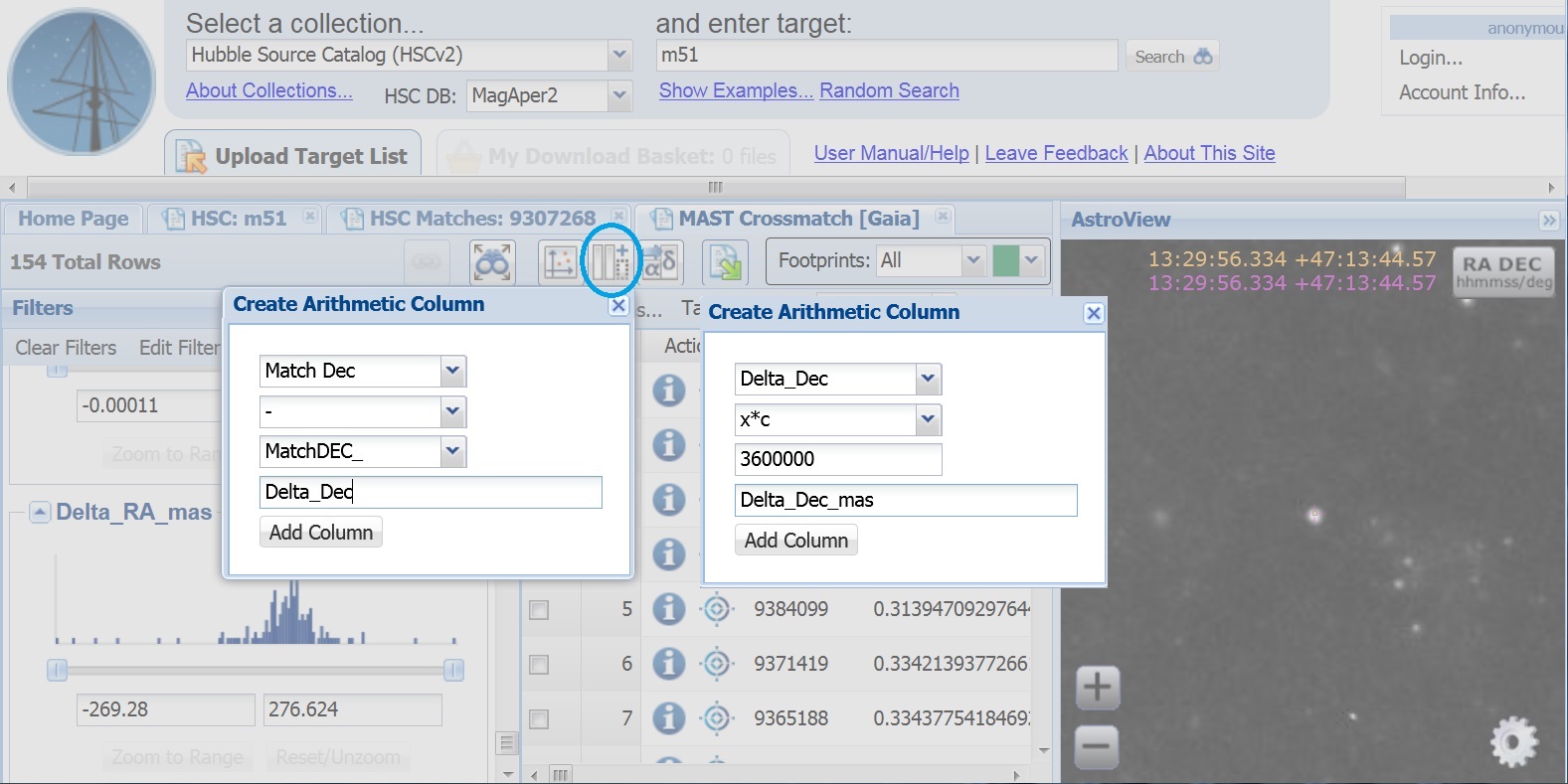
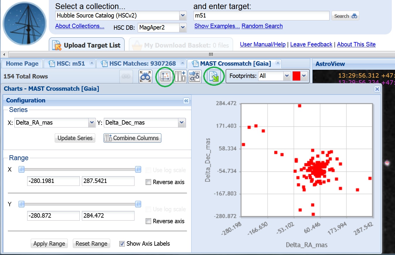
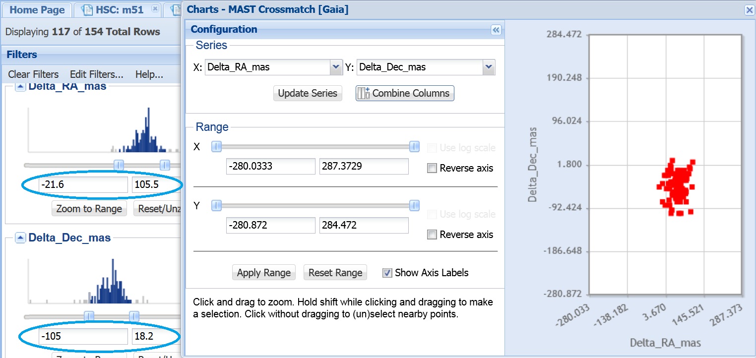
Then use the "View charts for these data" (blue) to plot, and set the X and Y series to be the Delta_RA_mas and Delta_Dec_mas columns. We find a nice concentrated knot of points from good matches of isolated point like objects, with a halo of outer points from regions that are crowded. We now find that the inner scatter ball has a declination diameter of about 100 mas (milli arcseconds). We will get a more precise value in steps below.
|
Step 6 - Download the table and calculate the means and standard deviations.
Download the table using the "Export the Data to a local file"
Average (Delta_RA) = 41.9 + 63.5 mas |
|
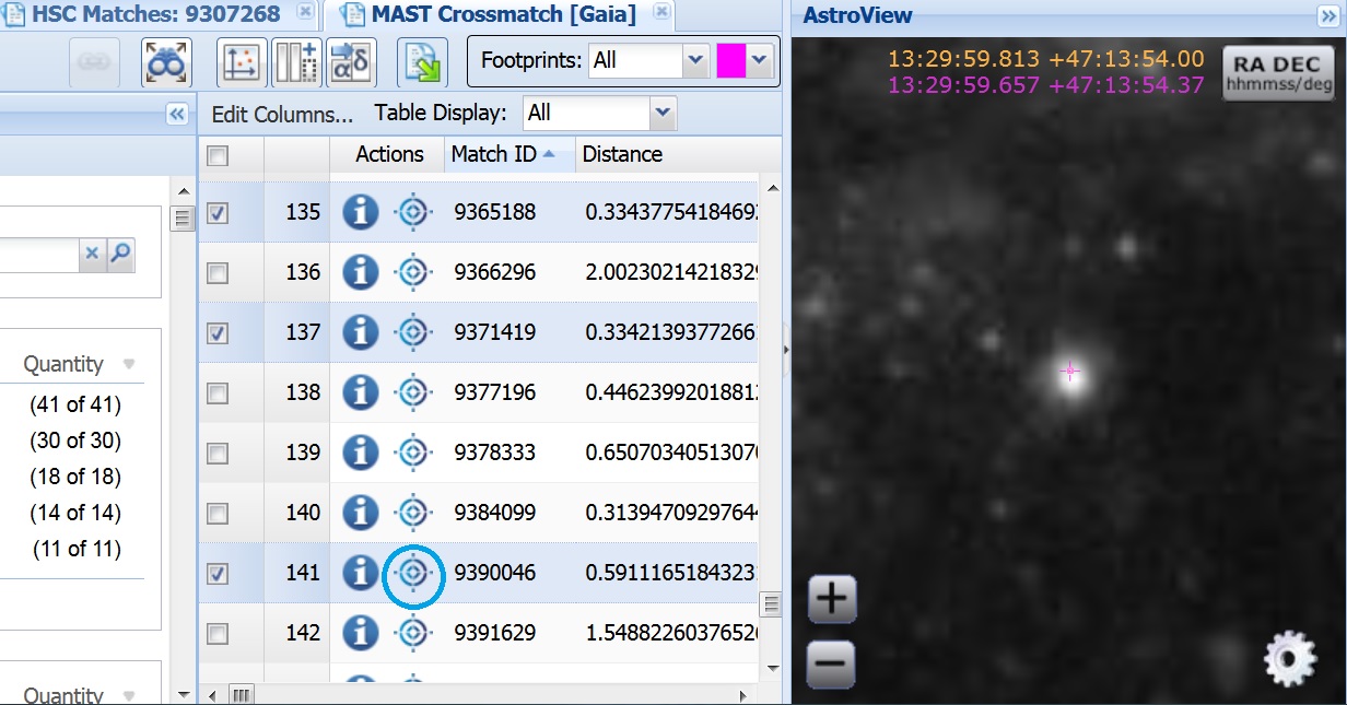
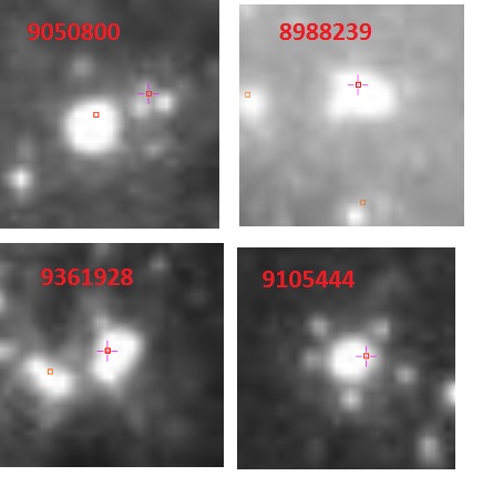
Step 7 - Select 5 of the more reliable matches and recompute.
If we pick 5 of the best (isolated, single) looking matches around
object 9307628 (i.e., 9307628, 9355644, 9371419, 9365188, 9390046 -
click on the bullseye |
The light colored points in this figure show the smaller scatter.
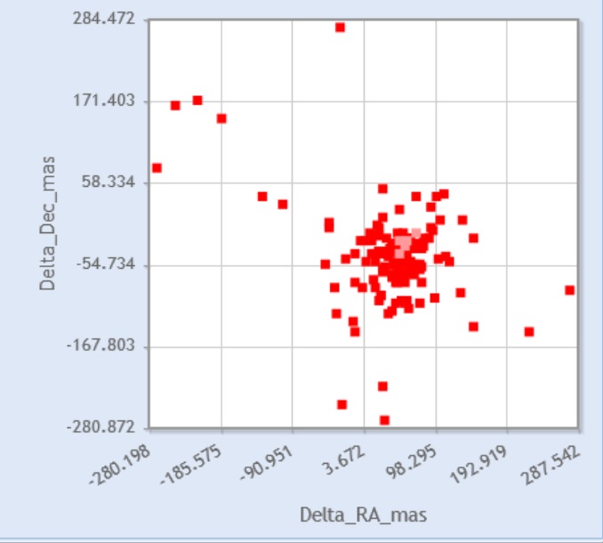
Doing a similar exercise in other small parts of the image result in similar spreads, but centered at slightly different parts of the scatter ball. Hence the fairest thing is to pick a slightly larger range that encloses the entire core which would represent the astrometric accuracy across the full image.
If we look at some of the objects that are more than 1 sigma from the average, we see that they are blended objects, which explains why there are far from the average.
We will exclude points greater than 1 sigma from the average (blue); note that I have converted from decimal degrees to mas. This results in keeping 117 of the original 154 matches, and gives scatters of 24 mas for RA and 25 mas for Dec. Since our requirement is that the HSC coordinates be in the JWST Guide Star (GAIA) reference frame to with ~20 mas, we can use the HSC to define our JWST observation.
|
Step 8 - Add the offsets to the HSC to align with GAIA. There is a significant shift between the HSC and GAIA reference frames, with an RA shift of 48.0 mas (the full set gave 41.9 in step 6) and -45.1 mas in Dec (the full set gave -43.4 mas). So, we must add these offsets to our coordinates for the entire sample of M51 targets (the MSC:m51 page) using steps similar to Step 5. Note that the offsets, in decimal degrees, are 2.00E-05 in RA and -1.25E-05 in Dec. |
|
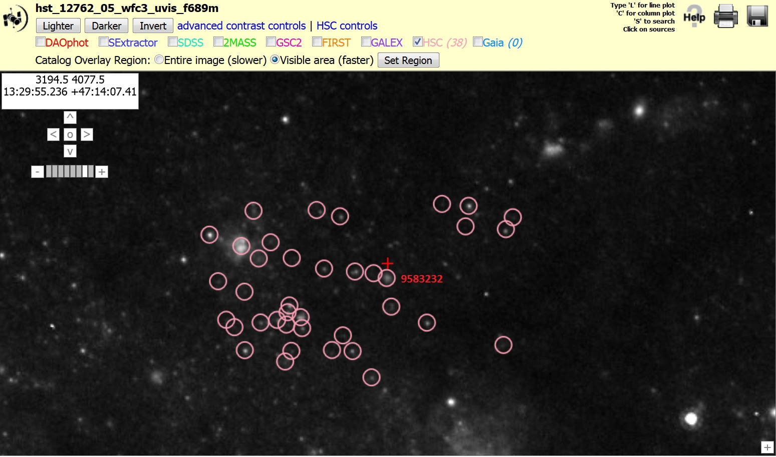
Step 9 - Select some clusters to use for JWST observations. We now add a set of cluster candidates which are the program objects we want to observe with JWST. We reset the magnitude range for F689M to use all the objects, and select a range in Concentration Index with CI = 1.6 to 2.2 (blue), appropriate for slightly resolved clusters (stars are normalized to have CI = 1.0 in the HSC). |
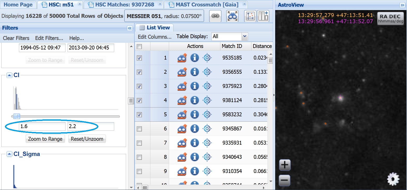
We click on the following objects that look isolated
and diffuse:
9535185, 9356555, 9375923, 9381124, 9583232
and they are moved to the top of the list.
The fact
that these are slightly resolved can be seen using the HLA interactive
display (see Step 3).
Note that in the next version of the HSC (version 3), there will be a dramatic improvement to the HSC astrometry, as the HSC will use the new PanStarrs coordinates which have been normalize to GAIA and have about 10 rather than 100 mas absolute astrometry. Hence, the need to add an offset may go away.
 icon
(
icon
( icon
for the fourth
object (9307268) (
icon
for the fourth
object (9307268) ( icon
(
icon
( icon
(
icon
( icon (
 icon (
 icon (