FUSE was designed to provide high resolution spectra (λ/Δλ ≥ 20,000) with large effective area (20 -70 cm 2) across the 905 - 1187 Å FUV spectral bandpass.
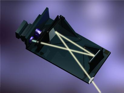
The FUSE satellite consisted of two primary sections: the spacecraft bus and the scientific instrument. Integrated, these components stood 18 feet (5.4 m) tall and weighed just under 3000 lbs. (1360 Kg). The payload is shown at Kennedy Space Center in June 1999 in Figure 2‑1 (left). A schematic of the light path for the science instrument is shown in Figure 2‑1 (right).
The challenge of designing a high-throughput FUV instrument and maintaining it throughout the lifetime of the mission was met by adopting a design that minimized the number of optical elements, employed a large-format, low-background detector, and retained throughput through vigilant maintenance of a tight contamination control plan and operational strategy to avoid degradation of the mirror coatings.
The resulting FUSE science instrument consisted of four separate telescopes and spectrographs. Each of the four FUSE telescopes was comprised of a co-aligned, normal incidence, off-axis parabolic primary mirror that illuminated a separate Rowland circle spectrograph channel equipped with a holographically-ruled diffraction grating that illuminated one of the two FUV microchannel plate (MCP) detectors. The essential features of this design are illustrated schematically in Figure 2‑1. Each of the two delay line MCP detectors recorded spectra from a pair of optical channels. At the entrance to each spectrograph was a Focal Plane Assembly (FPA) that could be moved in both the tangential and radial directions with respect to the Rowland circle. Adjustable Mirror Positioning Assemblies (MPAs) along with the FPAs permitted co-alignment and focus of the four channels. Attitude determination for target acquisition and fine pointing guidance data was provided by one of the Fine Error Sensor (FES) CCD (slit jaw) cameras operating in the visible on two of the four channels. The prime advantages of this design of four independent UV optical paths was that it permitted the optical coatings to be tailored to maximize instrument effective area across the FUSE bandpass, and that a high effective area could be combined with good aberration control in a package that would fit into the fairing of a practical launch vehicle. Some basic properties of the FUSE instrument are summarized in Table 2.2‑1 and Table 2.2‑2. Only ranges of effective area and spectral resolution are shown for each channel/segment; see Figure 4‑4 for plots of the effective area as a function of wavelength and Figures 4-2, and 4-3 for the spectral resolution as a function of wavelength.
Active thermal control and science instrument operations were performed by the Instrument Data System (IDS) computer. Instrument power was obtained from the spacecraft and was managed by the Instrument Power Switching and Distribution Unit (IPSDU) for instrument subsystems.
| Channel | SiC1 | LiF1 | SiC1 | LiF1 |
| Detector Segment | A | A | B | B |
| Wavelength Range [Å] | 1090.9 - 1003.7 | 987.1 - 1082.3 | 992.7 - 905.0 | 1094.0 - 1187.7 |
| Spectral Resolution | 12000-23000 | 10000-21000 | 10000-20000 | 11000-21000 |
| Plate Scale [arcsec/mm] | 84.4 | 84.4 | 84.4 | 84.4 |
| Inverse dispersion [Å/mm] |
1.03 | 1.12 | 1.03 | 1.12 |
| Effective Area [cm2] At launch |
5.5-9.0 | 3.5-28 | 6.0-8.5 | 12-28 |
| Effective Area [cm2] End-of-Mission |
2.5-5.0 | 3.0-24 | 2.5-5.0 | 8.0-21 |
Table 2.2‑1:
| Channel | SiC2 | LiF2 | SiC2 | LiF2 |
| Detector Segment | A | A | B | B |
| Wavelength Range [Å] | 916.6 - 1005.5 | 1181.9 - 1086.7 | 1016.4 - 1103.8 | 1075.0 - 979.2 |
| Spectral Resolution | 11000-19000 | 14000-23000 | 12000-20000 | 9000-19000 |
| Plate Scale [arcsec/mm] | 84.4 | 84.4 | 84.4 | 84.4 |
| Inverse dispersion [Å/mm] | 1.03 | 1.12 | 1.03 | 1.12 |
| Effective Area [cm2] At launch |
10-12 | 19-30 | 3.5-6.5 | 2.0-17.5 |
| Effective Area [cm2] End-of-Mission |
5.0-6.0 | 14-21 | 2.0-3.5 | 2.0-16 |
Table 2.2‑2: FUSE Instrument Specifications - Channel 2
2.3 Optical Design
The FUV instrument (see Figure 2‑1) consisted of four separate optical paths, or channels. Each channel was illuminated by its own normal-incidence, off-axis parabolic primary mirror with a Focal Plane Assembly (FPA), containing a set of three spectrograph apertures/slits, located at the focus of its telescope mirror. The four telescope primary mirrors were identical off-axis paraboloids, each with a rectangular 352 μm x 387 μm clear aperture, a 2245-μm focal length, and approximately 5.5° off-axis angle (Kennedy et al. 1996). At the focal plane, ~90% of the light in the point spread function (PSF) was within a circle of diameter 1.5 arcseconds. Each spectrograph was a Rowland circle design whose holographically-ruled diffraction grating illuminated a section of a FUV delay line detector. Figure 2‑1 (right) illustrates the detector multiplexing layout whereby two channels (one SiC and one LiF) illuminate different areas on a single detector. The channels had to be co-aligned so that light from a single target properly illuminated all four channels, thereby maximizing the throughput of the instrument. This co-alignment was accomplished with actuators on the mirror assemblies and the FPAs.
 | 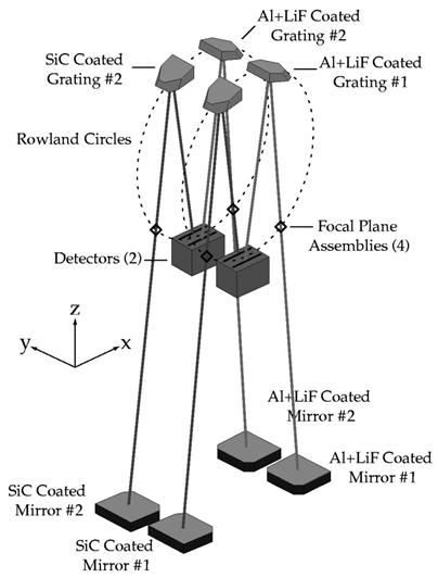 |
Figure 2‑1: Left: The integrated FUSE satellite. Right: Optical layout of FUSE instrument showing 4 channel design but only two detectors.
The multi-channel aspect of the FUSE design was a key element in maximizing instrument throughput. It permitted the use of different optical coatings on different channels. Two mirrors and two gratings were optimized for reflectivity in the 905-1100 Å bandpass using an ion beam sputtered silicon carbide (SiC) coating over an evaporated aluminum layer. The aluminum layer lowered the emissivity of the surface permitting better thermal control. The reflectivity of the remaining two mirrors and gratings was maximized from 1025-1187 Å using lithium fluoride (LiF) over aluminum. SiC has nearly constant reflectivity (~30%) across the FUSE bandpass. The reflectivity of LiF/Al is low shortward of ~1025 Å then rises sharply to ~70% near 1200 Å (The FUSE Data Handbook 2009). The LiF/Al coatings provided approximately twice the reflectivity of SiC at wavelengths > 1050 Å, but very little throughput below ~1020 Å. Throughout this document the four channels will be referred to as either "the SiC channels" or the "LiF channels" according to their coatings and hence their performance characteristics.
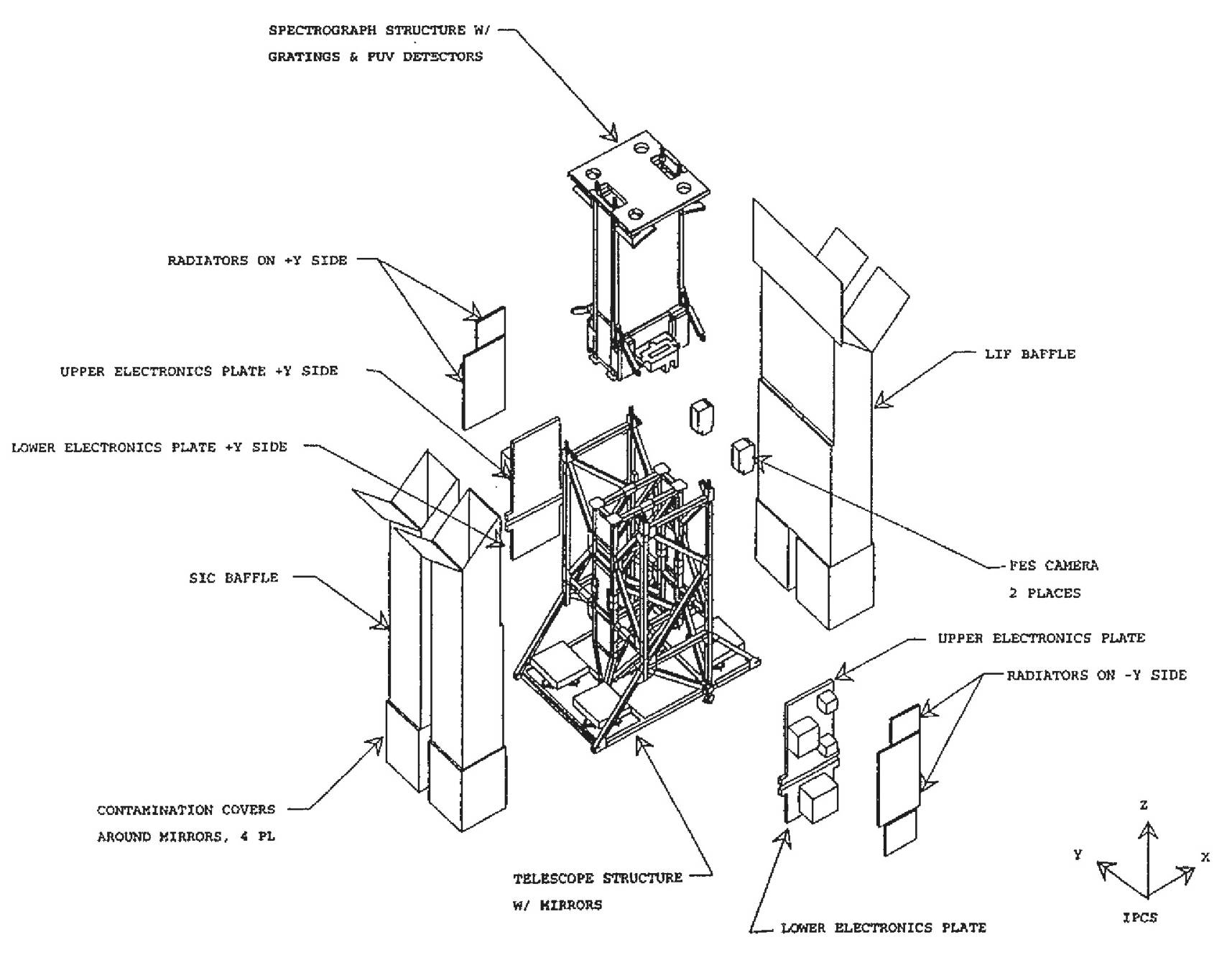
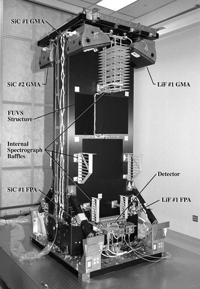
Figure 2‑2 : Exploded view of the FUSE instrument structure. This figure illustrates the relationship between the photograph of the assembled, flight-ready, FUSE instrument in the previous figure and the schematic of the optical layout of the telescope and spectrograph.
These four channels comprised two nearly identical "sides" of the instrument, where each side consisted of one LiF and one SiC channel. Each side of the instrument produced two spectra, one from each channel, that fell onto a single detector. Each channel had a band pass of about 200 Å requiring spectra from two channels to span the ~290 Å wavelength range of the instrument. All four channels covered the ~1015-1075 Å region.
The orientation of the instrument in the instrument prime coordinate system (IPCS: X, Y, Z) is shown in Figure 2‑1. The +X side of the instrument always pointed away from the sun throughout an orbit, while the –X side always pointed toward the sun. This orientation minimized the amount of sunlight that could make its way down the baffles surrounding the LiF channels, which were located on the +X (i.e. shaded) side of the instrument. Minimizing stray light in the LiF channels was crucial to the operation of the Fine Error Sensor (FES) guidance cameras, which operated at visible wavelengths on the LiF channels. To ensure that the radiator of the operational FES was kept in the shade, the satellite orientation was biased by several degrees in roll around the Z axis. These design and operational strategies succeeded in keeping Solar stray light to acceptable levels; however, when observing at low Earth-limb angles, stray light from the bright Earth could drown out all but the brightest guide stars. FES star field images acquired at orbit noon (Figure 4‑23) illustrate the impact scattered light in the FES guidance camera could have when attempting to acquire and track guide stars.
2.4 Focal Plane Assemblies
At the focus of each telescope mirror was a Focal Plane Assembly (FPA) that acted as the optical entrance aperture for each spectrograph channel (Figure 2‑3). The front surface of each FPA was a diamond milled, flat mirror with vapor deposited aluminum to provide a highly reflective surface in the visible. This optical flat mirror was mounted on a precision two-axis flight-adjustable stage. Light from the off-axis parabolic telescope entered the spectrograph through the four laser drilled FPA apertures (1.25" × 20", 4" × 20", 30" × 30", and a 0.5" pinhole, Table 2.4‑1) that had been cut into the flat. For ease of reference, the three primary apertures were dubbed HIRS, MDRS, and LWRS; the pinhole aperture was never located on orbit, and never used operationally. Although these apertures were offset in the direction perpendicular to dispersion, the apertures were not shuttered: all light (including the night sky and serendipitous targets) incident at an aperture was passed through the aperture to the grating, which then dispersed the light onto the detector. Since these apertures were offset in the spatial direction, light passed by each of the apertures was imaged onto a different section of the detector. The geometric arrangement of these apertures is shown in Figure 2‑4. The aperture plates were not mounted perpendicular to the telescope focal plane, but were rotated 10.8 degrees about the Y axis; the reflected beams in the LiF channels were directed into the corresponding FES cameras, and against the sides of the telescope baffles in the SiC channels.
For the LiF channels, light that did not pass through an entrance aperture was reflected by the mirrored surface into the FES visible light CCD camera system. Images of stars in the field of view (FOV) around the apertures were then used for acquisition and guiding by the FES, which provided feedback to the spacecraft attitude control system for stabilizing the pointing (Section 2.7). Only the LiF channels were equipped with FES systems, because the Al/LiF coatings on the telescopes were far more reflective in the visible than the SiC coatings and because a prime and backup system were considered to be sufficient.
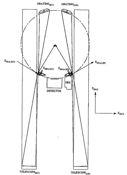
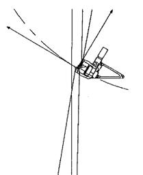
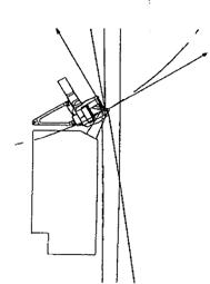
Figure 2‑3: Schematic of the LiF1 and SiC1 FPAs shown relative to the instrument optical design and beam size (top), with a detail of the FPAs and their relationship to the Rowland Circle and the IPCS coordinate system (bottom). In the LiF channel, light from the star field in the vicinity of the target is reflected into an FES camera.
| Aperture | Keyword | Dimension (arcsec) |
Y FPA position (arcsec) |
Comments |
|---|---|---|---|---|
| High resolution | HIRS | 1.25 × 20 | -10.27 | |
| Medium resolution | MDRS | 4.0 × 20 | +90.18 | |
| Low resolution | LWRS | 30 × 30 | -118.07 | Default Aperture |
| Pinhole | PINH | ~0.5 (diameter) | Not Used |
Table 2.4‑1: Apertures
This set of apertures was designed to permit the following functionality.
- The high resolution aperture (HIRS: 1.25 × 20 arcsec) passes ~70 % of the light from a centered point source (throughput as high as 90% has been measured, but 70% is more typical). The HIRS aperture was designed to maintain the highest resolution at the expense of photometric accuracy. This was the expectation even for perfectly stable optics. Because of the difficulties encountered with maintaining channel alignment on-orbit, this aperture was used sparingly during the mission.
- The medium resolution aperture (MDRS: 4 × 20 arcsec) provided maximum throughput (~98%) while minimizing airglow contamination. With stable mirror alignment, this aperture provided a spectral resolution that was only slightly reduced from the actual resolution achieved when using the HIRS aperture for a point source target. However, on-orbit thermal drifts of the channels with respect to the LiF guide channel resulted in limited use of this aperture due to the effort required to maintain alignment. Significant loss of the SiC channel data typically resulted with use of this aperture under nominal operations. The impact of on-orbit thermal drifts is discussed further in Section 4.2.
- The low resolution aperture (LWRS: 30 × 30 arcsec) was a large square aperture intended for observations of faint extended objects. It produced a filled-aperture resolution of about ~100 km/s. However, as a result of the on-orbit motion of the instrument channels with respect to one another, use of the LWRS was most likely to result in obtaining data in all channels. Consequently, the LWRS aperture became the preferred aperture for point source observations. The thermal motions had the potential to degrade the resolution, but this was limited by the short duration of HIST exposures and was corrected by CalFUSE for TTAG exposures; see Sections 2.8, 4.2.3, and 4.3.1 for details. For nominal operations, this was the default aperture.
- The pinhole aperture (PINH: approximately 0.5 arcsec in diameter) was not used on orbit.
Each of the four FPAs included precision actuators that permitted independent motion of the FPAs in two axes: tangential to the Rowland circle and along the radius. The FPAs could not be moved in the Y direction. FPA motion along the radius of the Rowland circle enabled focusing of the apertures with respect to the spectrograph grating and detector (Section 6.2).This was performed infrequently over the course of the mission. The motion tangential to the spectrograph Rowland circle was parallel to the dispersion direction and perpendicular to the apertures. Adjustments of the FPAs along this axis were used to compensate for small X-axis mirror motion misalignments (Section 4.2.3.1) and were often performed as part of the set up for an observation. They also permitted "focal plane split" (FP-split) observations to enable high signal-to-noise measurements of bright targets. FP-splits were performed by taking spectra at different FPA settings so that detector fixed-pattern noise could be smoothed out when the data were co-added. Different position patterns were used depending on the observation. Table 2.4‑2 shows the FPA locations at the nominal telescope alignment and the adjustments in position and corresponding telescope offset to place the target in the aperture for a typical FP-split observation. The FPAs had a 400um commandable range in X, at 12.63 μm/arcsec.
Table 2.4‑2
FP-split step
LiF1 FPA
Other FPAs
Slew Offset
Nominal position
117 μm
175 μm
0.0”
1
65 μm
123 μm
-4.1”
2
142 μm
200 μm
+2.0”
3
185 μm
243 μm
+5.4”
4
277 μm
335 μm
+12.7”
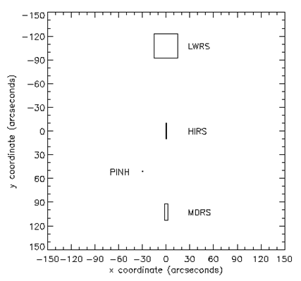
Figure 2‑4:
The locations of the FUSE apertures projected on the sky for a slit
position angle of 0°
with North in the -Y direction.
Positive aperture position angles correspond to a counter-clockwise rotation of
the apertures on the sky. In the FPA coordinate system the LWRS, HIRS, and MDRS
apertures are centered at Y= -118.07”, -10.27”, and +90.18”, respectively.
This diagram represents only a portion of the FPA; the full active area is
~19arcmin × 19 arcmin.
The Far Ultraviolet Spectrograph,
FUVS, had four spectrograph channels: one for each of the four telescope channels
(Figure 2‑1). Each spectrograph channel was conceptually similar to a Rowland
circle spectrograph, except that aberration corrected, holographically-ruled,
gratings were used to control the astigmatism typically encountered in a
Rowland system. Light from the diverging f/5.3 telescope beam passed
through an FPA aperture at the telescope focal plane and entered into the
spectrograph cavity. The beam was then incident on one of the four diffraction
gratings, which focused the spectra onto one of two, double delay line MCP
detectors. The gratings were paired so that a single detector had
spectra from both a SiC and a LiF grating spatially offset from each other.
Because of the multiple apertures, there were typically three spectra from each
channel projected onto a single detector. The grating
substrates were fused silica with 270mm × 265mm rectangular apertures. The
concave grating surfaces were holographically-ruled aberration-corrected
spheres with a radius of curvature of 1652mm. The holographic recording
parameters were optimized to reduce the astigmatism from approximately 60 mm
(using standard parallel groove gratings) to less than 1 mm while maintaining
resolution. This dramatically increased the sensitivity of the instrument. The
characteristic groove densities were 5767 grooves/mm for the SiC-coated
gratings and 5350 grooves/mm for the Al/LiF-coated gratings (Wilkinson et. al.
1998, and references therein). This resulted in a reciprocal linear
dispersion of 1.03 Å/mm for the SiC channel and 1.12 Å/mm dispersion for the
LiF channel. Coupled with the detector pixel size, this resulted in a
scale of 6.2 mÅ/pixel for the SiC channel and ~6.7 mÅ/pixel for the LiF
channel, in the dispersion direction. Selected design parameters for the spectrograph
and diffraction gratings are listed in Table 2.5‑1.
The
diffracted light then focused onto the double delay line, MCP detectors. Each
detector had an active area of 190 mm
× 10 mm that was divided into two 85 mm
× 10 mm MCP stacks,
referred to as the A segment and the B segment. The MCPs were curved to 826 mm
and a potassium bromide (KBr) photocathode was applied to the top MCP plates to
enhance the detection quantum efficiency in the FUV. The average resolution of
the FUSE detectors is 25 μm in the
spectral direction and 50-60 μm in the
spatial dimension. The FUSE detectors are described further in sections 2.6 and
4.4. Table 2.5‑1: Spectrograph and Grating Properties
Figure 2‑5: Photograph of the FUVS in a clean room at
University of Colorado Boulder just prior to shipment to Johns Hopkins University,
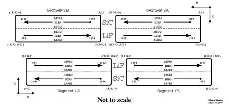
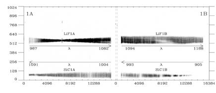
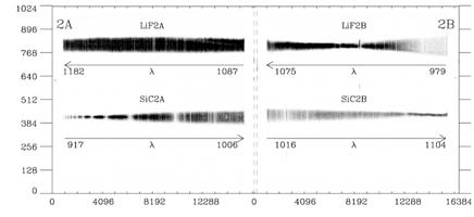
with the major optical components identified. The FUSE spectral range extended
from about 905 Å to 1187 Å. Each detector had one SiC spectrum and one LiF
spectrum imaged onto it, and therefore covered the entire wavelength range. The
two channels were offset on the detector perpendicular to the dispersion
direction to prevent the spectra from overlapping. The dispersion for the
SiC and LiF spectra were in opposite directions from each other
(Figure 2‑6). Each detector was divided into two functionally independent segments (A
and B) separated by a small gap. To ensure that the gaps did not fall at the
same wavelength region in both detectors, they were offset slightly with
respect to each other. Table 2.5‑2 lists the wavelength coverage of each of the
eight detector segment/channel combinations. Nearly the entire wavelength
range is covered by more than one channel, and the important 1015–1075 Å range
is covered by all four, providing the highest effective area and the greatest
redundancy. Table 2.5‑2: Wavelength Ranges for Detector Segments
The FUSE spectrographs were based
on the highly efficient Rowland circle design. The holographically-ruled
gratings partially corrected the inherent aberrations in this design, but the
remaining astigmatism restricted spatial imaging capabilities. The image of a
point source had a vertical extent of 150 to 1100 μm (~14 to 100 arcsec) on the
detector, depending on wavelength. In comparison: the height of the HIRS and
MDRS apertures were 20 arcsec, or 220 µm projected on the detector, smaller
than the astigmatic height of a point source image at most wavelengths. The
astigmatism of the FUSE optical system was corrected near the O VI line for LiF
spectra, and near 920 Å and 1090 Å for the SiC spectra (Figure 2‑7).
Differences in alignment, fabrication, etc. for the
two sides, resulted in slightly different locations for the minimum height. The
approximate wavelengths at which the astigmatic correction points occurred
were: 916 Å (SiC1B), 926 Å (SiC2A), 1026 Å
(LiF1A), and 1036 Å (LiF2B).
Figure 2‑7: The astigmatic height of the FUSE spectra are shown in these figures. The units of
both axes for both the top and bottom figures are detector elements, or pixels.
A small portion of an H2
spectrum recorded by flight detector segment 1B during Spectrograph I&T at
the University of Colorado is shown in Figure 2‑8. A number of
interesting characteristics of the spectral design and the test configuration
are illustrated in this Figure. First, note that the spectral resolution
degrades with the width of the aperture. This is due to the fact that the
aperture was fully illuminated during the test. Emission from large extended
sources (e.g. supernova remnants, planetary nebulae, galaxies, etc.) exhibited
this dependence of spectral resolution on aperture width. Under
conditions of nominal pointing accuracy and jitter, a point source spectrum
would have roughly the same spectral resolution in all apertures. Second,
notice the astigmatic height and curvature of the spectra in the LiF channel
(the upper 3 spectra). This is a natural consequence of the optical
design. The narrow aperture is on-axis, and the spectrum through this slit is
symmetric about the dispersion axis. Note that the other two LiF spectra
are asymmetric since they are off-axis. The spectrum through the MDRS aperture
(the top spectrum) is tilted slightly to the left while the spectrum through
the LWRS (the 3rd spectrum down from the top of the image) is tilted to the
right. The SiC spectra all have much smaller astigmatic heights because
the spectra are nearer to a holographic correction point at these wavelengths.
Comparison of the widths of the LiF and SiC spectral lines clearly illustrates
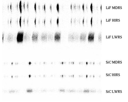
the fact that the spectral resolution is lower at a spatial focus point. Figure 2‑8: Molecular
hydrogen emission spectrum recorded by detector 1B. This figure shows the full
extent of the segment in the Y direction (1024 pixels) but only a very small
extent in X (1000 pixels or about 6 Å). This image was constructed
by adding together 6 different images, each made with the lamp source
illuminating an individual aperture. From the top to the bottom of the
image, the spectra are LiF (MDRS aperture), LIF (HIRS aperture), LiF (LWRS
aperture), SiC (MDRS aperture), SiC (HIRS aperture), and SiC (LWRS
aperture). The pinholes were not illuminated. The LiF spectra
are centered at ~1160 Å while the SiC spectra are centered at ~930 Å.
The FUSE instrument included two
Double Delay Line (DDL) detectors which collected incoming photons and measured
their positions. Three FUV detectors were built at the Space Sciences
Laboratory at the University of California, Berkeley. Unit FL01 remained on the
ground as a spare and was later used for ground testing, while units FL02 and
FL03 were used in the instrument as Detector 1 (side 1 of the instrument,
collecting photon events as part of the SiC1 and LiF1 channels) and Detector 2
(SiC2 and LiF2), respectively. The three detectors had identical physical
characteristics, and were designed to be as similar as possible. Differences
between them are due primarily to differences in the microchannel plates (MCPs)
and the adjustments of the electronics to account for those variations. The
differences in wavelength coverage between side 1 and side 2 of the instrument
were determined by the mounting locations on the Rowland circle. Each detector consisted of two
segments. Mechanically, each detector was a single unit; electrically each
segment was unique with most of its own electronics. Keeping the segments
separated permitted each to be individually optimized. In addition, it ensured
that a problem with one segment did not prevent its companion from being
operated normally. Thus, if desired one detector segment could be operated
normally while the high voltage on the adjacent segment was turned off. Light coming from one of the FUSE
gratings to the detector first passed through a 95% transmission, +15 volt ion
repeller grid, then through a 95% transmission ‘QE Grid’ designed to improve
the quantum efficiency of the system, before reaching the KBr-coated MCPs. The
photons striking the photocathode were converted to electrons via the
photoelectric effect, multiplied as they passed through the stack of three
(Z-stack) MCPs, then proximity-focused onto the DDL anode. The DDL electronics
determined the location of each charge cloud by measuring the time it took for
the charge to propagate along the anode (for the X, or dispersion direction) or
by charge division (for Y, or cross-dispersion). Thus, the reported positions
of detected photons do not represent physical pixels, as would be the case for
a CCD detector, but rather are digitized representations of analog
measurements. The measurement process and implications for the data are
described in subsequent sections. The top-level detector specifications are
summarized in Table 2.6‑1.
Table 2.6‑1: Detector Specifications
Each detector subsystem was
divided into three interconnected, modular assemblies. These were the Vacuum
Assembly, Electronics Assembly, and Stim Lamp Assembly. The Vacuum Assembly was
mounted in the spectrograph cavity and contained the detector imaging elements
(grids, MCPs, anode, etc.) in a stainless steel vacuum housing, along with a
high voltage filter module, charge amplifiers, timing amplifiers, a motorized
door and mechanism, and ion pumps to maintain a high vacuum inside the vacuum
box before launch. The Electronics Assembly, mounted to the instrument
electronics baseplate in the electronics cavity, included the low- and
high-voltage power supplies, Time-to-Digital-Converters (TDCs),
Charge-to-Digital-Converter (CDCs), and a Data Processing Unit (DPU), along
with an interface to the instrument computer – the Instrument Data System
(IDS). The Stim Lamp Assembly consisted of a mercury vapor lamp that was mounted
to the spectrograph structure inside the spectrograph cavity and was powered
and controlled via the detector electronics. Details on each of these
assemblies are given in the sections below. Each detector subsystem included
thirteen thermistors to monitor the temperature of the detector hardware.
Although the temperatures of the anode and some parts of the electronics were
known to affect the data, the thermistor information was only used as a general
diagnostic, and detector stim pulses, described below, were used to account for
temperature effects in the data. The detector Stim Lamp Assemblies
(one for each detector) allowed direct, quasi-uniform illumination of each
detector, with count rates of ~2,000 to ~12,000 counts per second, depending on
the segment. These stim lamps were designed to provide general diagnostics of
detector health. They were not designed to provide a true flat field of the
detectors. Each stim lamp assembly included
the mercury vapor stimulation (or “stim”) lamp, a mounting bracket, and a
pinhole aperture to coarsely control the amount and direction of light reaching
the detectors. They were mounted to a structural bracket in the spectrograph
cavity, approximately 1.25 meters from the detectors. Before launch, the lamps
were used to provide detector aliveness tests while the instrument was at
atmospheric pressure by illuminating the MCPs through the sapphire windows in
the vacuum doors. On orbit, they were used regularly throughout the mission as
a means of monitoring detector performance, especially gain sag (Section 4.4.2.
The stim lamps were powered
through the detector auxiliary power supply, which also powered the ion pumps. The fine pointing of the FUSE
satellite was achieved by using the FES, a visible light imaging camera. The
primary functions of the FES were to (1) image the focal plane in order to
acquire a target, and (2) provide the fine pointing guidance data to be used by
the spacecraft attitude control system to maintain accurate pointing during
science observations. Two FES cameras were included onboard FUSE. One FES was
used at any given time with the second as a backup. Each FES directly viewed the
focal plane of one of the FUSE primary mirrors. The prime FES unit (FES-A) was
mounted just below the FPA (Focal Plane Assembly) in the LiF1 optical channel,
so that the mirrored surface of the FPA slit-plate redirects the light into the
FES where it is reimaged onto a CCD detector. A schematic view of the LiF1
light path is shown in Figure 2‑3 and Figure 6‑33. The redundant FES (FES-B)
was similarly mounted in the LiF2 channel. A complete visible-light subsystem
consisted of an FES, an FPA, a primary mirror, and the baffle tube assembly
that protected the optics from stray light. Each FES was composed of
three subassemblies: the camera assembly, containing the optics, CCD detector,
and preamps; the controller assembly, containing all the remaining electronics
and external electrical interfaces, and a radiator and heat strap used to cool
the CCD.
The optical system consisted of
two off-axis aspherical mirrors, a filter wheel, and a doublet lens. Figure 2‑9 shows a schematic illustration of the light path
inside the FES. The FES imaged a field of view of 21′ × 21′
onto the surface of a CCD detector, which
was reduced to a usable area of 19.3′ × 18.3′
by an aperture mask located at the surface of each FPA mirror. The point spread
function (PSF) of the system had a typical full-width at half maximum (FWHM) of
about 2 pixels (~ 5″ ) everywhere in the field of view,
consistent with the original design and pre-flight measurements, and ideal for
centroiding with sub-pixel accuracy. The system throughput was also consistent
with pre-flight estimates: a typical V = 13.5 mag star produced a signal
of 9350 e-/sec. Table 2.7‑1 summarizes the
characteristics of the FES. Distortions across the FOV were
small, at most 1.5% in the far corners of the FOV. The distortions for FES-A
were measured during in-orbit checkout and polynomial corrections were uplinked
to the IDS. A more extensive set of calibration observations was performed for
both cameras in late 2001, which significantly improved the residuals in the
corners of the field. Imperfections in the optical
surfaces and obstructions in the light path (such as mis-aligned baffles) would
scatter and diffract light from sources in the FOV. This limited the ability of
the system to detect and track faint guide stars when very bright objects were
present in the FOV. Initial tests showed that the IDS could identify star
fields and track on guide stars at the nominal faint limit when stars as bright
as V = 1.5 mag were present in the FOV. Using special procedures (such
as performing initial acquisitions at offset fields) we were able to acquire
and track when much brighter objects were present, without having to use the
attenuating filter in the FES. This performance was much better than was
expected prior to launch. No internal focus adjustment
mechanisms were included in the FES, due to the cost and schedule constraints,
the limited volume available for the camera assembly, and because a limited
range of focus adjustment (100 microns) was expected to be required. Instead,
the choice was made that the optical design had to produce a PSF that was
insensitive to the expected changes in focus, and that the FES would have to be
carefully aligned and focused at the time it was installed on the telescope. A three-position filter wheel was
located between the FES secondary mirror and the doublet lens. The filters
incorporated in the filter wheel were a clear filter, a neutral filter for use
with very bright objects, and a broadband filter (red in one FES, blue in the
other). Once it was determined, early in the mission, that the neutral
density filter was not needed for acquisitions of bright objects, the FUSE
operations team decided to keep the filter wheel in the clear filter position,
and not to turn it. Given the critical role of the FES for fine pointing the
observatory, the FUSE operation team recognized that a malfunction of the wheel
could jeopardize the pointing of the observatory. Consequently, the neutral and
broadband filters were never used during the mission. Figure 2‑9 Table 2.7‑1: FES Camera Characteristics
The CCD detector was 1024 ×
1024 pixel thinned backside-illuminated CCD
mounted on a 2-stage thermo-electric cooler (TEC) and sealed in a kovar package
with a fused silica window. The CCD quantum efficiency, full-well depth,
charge-transfer efficiency, dark current, and readout noise were all in accord
with pre-flight measurements. The CCD was cooled using an external radiator in
combination with the TEC. Basic characteristics of the CCD are given in
Table 2.7‑2.
Table 2.7‑2: FES CCD Characteristics
The FES provided two types of data: images of the field of
view, and centroided positions of up to six selected stars. This information
was transferred to the FUSE Instrument Data System (IDS) which used this
information to 1) identify the field of view of the planned science observation
and move the target in the desired spectrograph aperture, and 2) to acquire and
track on guide stars during the observation in order to stabilize the line of
sight. The target recognition and fine guidance of the FUSE attitude control is
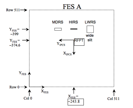
described further in Section 6.5.2 and by Ake et al. (2000). The locations of the FPA
apertures in the FES image and the relative orientation of IPCS coordinates and
raw FES-A pixel coordinates are depicted in Figure 2‑10. FES-B is
similar, except that the X-axis in FES-B is inverted: a corresponding image for
FES-B would have CCD column 0 on the right and column 511 on the left. Table 2.7‑3
gives the aperture and Reference Point positions in FES pixel coordinates. The
Reference Point is not a physical feature on the FPAs, but is an arbitrary position
offset from the apertures used in the target acquisition process; see Section 8 for additional information on coordinate conversion. FES images taken during the
identification process or at the end of an observation for the purpose of
pointing verification are archived at MAST as part of the science program
observation (see Section 5.1 of the
FUSE Data Handbook (2009) for additional information). Conversion from the FES
image coordinates to the world coordinate system is discussed in Section 8. HIRS 247 398 252 425 LWRS 289 398 209 425 RFPT 243.8 374.6 256.0 399.0 Table 2.7‑3: Center Positions of the Three Apertures
and the Reference Point in FES-A and FES-B 1 × 1-binned Images.
Figure 2‑10:
Diagram of an FES-A image with
its different coordinate frames. The raw FES CCD coordinates are (XFES,
YFES) with its origin at the lower left corner of the image. The FES
IPCS coordinates as projected onto the sky are (XIPCS, YIPCS)
with its origin located below the HIRS aperture. The exact location and size of
the three apertures are not to scale.
The IDS was the primary computer of the FUSE
science instrument. It was a fully redundant, programmable processor that
provided command and data handling functions for all other subsystems in the
instrument. The main functions performed by the IDS include:
1) processing,
management, and storage of science data from the FUV detectors
2) commanding the FES,
computing fine pointing measurements from stellar positions and images
generated by the FES, and transmitting the results to the spacecraft ACS;
3) managing instrument
thermal control;
4) synchronizing time
with the spacecraft;
5) running a script
engine, that provides absolute time and relative time commanding, and
rule-based autonomy capabilities for both scripted operations and health and
safety monitoring.
Only the first of these items is described here;
the other items are discussed in Sections 3 and 6.5
The IDS detector manager was a task designed to
read science data from the detectors and then process and store the data as
quickly as possible. The manager operated in either of two modes: address
stream (also called time-tag or TTAG) or spectral imaging (also called histogram
or HIST). These modes were selected for a specific exposure by the Mission
Planning system, typically based on the expected brightness of the target.
In address stream mode, raw detector data were
saved in a software FIFO in bulk memory. The IDS inserted time markers
into the data stream as the data were ingested. The default rate for inserting
markers was 1 Hz, but the rate could be set as high as 125 Hz. These markers
were accurate to 8 ms. The maximum rate at which the IDS could ingest data in
this mode was 8000 events/sec. The FIFO was readout continuously as the
exposure was taken. The maximum readout rate was roughly 3500 events/sec, lower
than the maximum ingest rate. Thus, once the FIFO filled the effective
data acquisition limit in TAG mode was 3500 events/sec. The issues affecting
the overall system deadtime are discussed in Section 6.9.
Observing in time-tag mode allowed the data to
be taken at full detector sampling (6 μm in X and 9-16 μm in Y), along with
photon event pulse height values. This permitted CalFUSE to perform
sophisticated filtering and corrections when extracting the resultant spectra.
Spectral shifts on the detector, either by grating or image motion (Sections 4.3.5,
4.2.3) or pointing instability (Sections 6.5.2 and 7), were removed by modeling
or using additional engineering telemetry. Doppler smearing and shifts in areas
of high gain sag (Section 4.4.2.1) were also corrected. Periods of detector
related problems, such as anomalous HV levels and event bursts (Section 4.4.3.3)
were edited out. Finally, in time-tag mode data from the entire active area of
the segments were downlinked, providing spectra through all apertures for
extended sources.
Histogram mode was used when the expected count
rate of the target exceeded 2500 counts per second. This mode allowed brighter
targets to be observed, but with certain disadvantages. The data were binned by
8 pixels in Y and most of the temporal corrections available for time-tagged
exposures could not be made. Doppler smearing was minimized by keeping the
exposures short (~< 7 minutes). In this mode, the IDS accumulated an image
of part of the detector in bulk memory by computing an array location from the
detector raw coordinates and incrementing the number of counts in that
location. Only limited portions of the detector could be stored in the IDS in
this mode, as a result of memory size limitations. The regions to be stored
were defined by the Spectral Image Allocation (SIA) Tables, which are described
in Section 6.3.3. The maximum event rate that could be ingested by the IDS in
this mode was 32,000 events/sec.
At the end of the exposure, the image was read
out. The IDS appended an 8 character observation ID and 3 character exposure
number assigned by the Mission Planning system to the downlinked packets. While
the exposures were in progress, periodic engineering snapshots of instrument
telemetry were taken to assist in the processing of the science data on the
ground. At a minimum, a snapshot was obtained at the beginning and end of the
exposure, and usually every 5 minutes during a longer integration.
A description of other IDS functions is
presented in Section 5 and a more detailed description of the
IDS is given by Heggestad & Moore (1999) and Artis et al. (2000). Further
information about CalFUSE processing of time-tag and histogram exposures can be
found in Section 4 of the FUSE Data Handbook 2009
and Dixon et al. (2007).
Next: Instrument Design Previous: Introduction Table of Contents
2.5 Spectrograph
2.5.1 Optical Design
Property
SiC
LiF
Rowland Circle diameter
1652
1652
Ruling density at grating ctr.
5767 mm
5350 mm
Grating (a)
24.0°
25.0°
Grating angle (b)
9.31660° at 986 Å
9.76612° at 1107 Å
Grating dimensions
260 mm (dispersion) × 275 mm (spatial)
Grating type
First generation, type II holographic
2.5.2 Wavelength
Coverage and Dispersion
Channel
Segment A
Segment B
SiC1
1090.9 - 1003.7 Å
992.7 - 905.0 Å
LiF1
987.1 - 1082.3 Å
1094.0 - 1187.7 Å
SiC2
916.6 – 1005.5 Å
1016.4 – 1103.8 Å
LiF2
1181.9 – 1086.7 Å
1075.0 – 979.2 Å
2.5.3 Spectral Image
Characteristics
2.6
Detector Design and Operation
2.6.1 Hardware and Software Description
Specification
Description
MCP pore size
(pore diameter / center-to-center spacing) 10 μm / 12.5 μm (top & bottom plates)
12.5 μm / 15 μm (middle plates)
MCP pore bias angle
13°
MCP Configuration
Z-stack
MCP size
95 μm x 20 μm, 80:1 L/D
MCP resistance
< 30 MΩ
Anode Type
Double Delay Line
Photocathode
KBr
Ion Repeller Grid
95% transmission, 1247 x 1247 µm spacing, flat
QE enhancement Grid
95% transmission, 1042 x 1009 µm spacing, curved to match MCPs
QE in FUSE bandpass
14 – 30%
Active Area
85 x 10 μm x 2 segments ~7 μm gap between segments
Curvature of front surface of MCPs
826 μm radius
Number of Pixels
16384 x 1024 per segment
Pixel size
6 µm x 10–17 µm, depending on segment
Detector resolution
~20 µm x ~80 µm
Lifetime Specification
> 107 events per 103 µm2
2.6.2 Stim Lamp Assembly
2.7
Fine Error Sensor Cameras
2.7.1
Camera Assembly
2.7.1.1 Optics
FES Properties
Value
FOV
19.3 ′ × 18.3′
Photometric bandpass
4000 - 9000 Å
Plate Scale
2.55" / pixel
Noise Equivalent Angle (typical)
≤ 0.15"
Sensitivity (typical)
9350 e- / sec @ V = 13.5
PSF
5" FWHM
Exposure time
0.048 – 300 sec
Subimage
3 – 25 pixels square
Centroid rate
6 10 × 10 subimages @ 1Hz Texp = 0.4 s
4 16 × 16 subimages @ 1Hz Texp = 0.4 s
6 16 × 16 subimages @ 0.5Hz Texp = 1.2 s
2.7.1.2
FES CCD Detector
CCD Properties
Value
Pixel Size
24 μm
Read Noise
7 e-
QE
55% @ 400nm, 65% @ 700nm, 37% @ 900nm
Gain
5 e-/ ADU
Full Well
280,000 e-
Digitization rate
50 Kpixels/sec
Parallel Clock rate
5,000 lines/sec
Dark current (MPP)
4.1 e- /pixel/sec at -30C (preflight)
Dark current (MPP)
33 e-/pixel/sec at -32C (1 yr post-launch)
2.7.2 FES
Images
FES-A
FES-B
Aperture
XFES
(pixel) YFES
(pixel) XFES
(pixel) YFES
(pixel)
MDRS
207
398
292
426
2.8
Instrument Data System (IDS)